Compare EchoPro and Echopop reports

Compare EchoPro and Echopop reports#

Visualizing year-specific differences#

The reports.compare module is used to visualize differences between reports produced by EchoPro and Echopop. These visualizations can be broken down into two major types:

Tables: quantities distributed across a non-geographic grid.
Geodata: quantities distributed spatially along the survey extent.

Along with importing the module, several variables can be pre-defined for convenience, but can also be manually defined for each and every function. This comprise:

ECHOPRO_REPORT_ROOT: The root directory for the EchoPro reports.
ECHOPOP_REPORT_ROOT: The root directory for the Echopop reports.
SAVE_FILEPATH: The directory where all figures will be written.
SHOW_PLOT: A boolean argument that defines whether to render the plot after (optionally) saving.

To examplify this module’s usage, the 2019 dataset will be used and is therefore initialized via:

from echopop.reports import compare
from pathlib import Path

ECHOPRO_REPORT_ROOT = Path("C:/Data/EchopopData/file_all_years_update_20260303/2019/output_echopro")
ECHOPOP_REPORT_ROOT = Path("C:/Data/EchopopData/file_all_years_update_20260303/2019/output_echopop")
SAVE_FILEPATH = Path("C:/Data/EchopopData/file_all_years_update_20260303/2019/notebook_dump")
SHOW_PLOT = True

Haul-based reports#

The aged- and total-length haul count reports are ingested using the read_pivot_table_report function, which has only a single argument:

filepath: The filepath for the haul-based report.

The output of read_pivot_table_report is a dictionary of multi-index pandas.DataFrame objects specific to sex="female", sex="male", and sex="all". Each pandas.DataFrame is then independently visualized via the plot_haul_count_comparisons with arguments:

echopro: The dictionary of EchoPro DataFrames.
echopop: The dictionary of Echopop DataFrames.
save_filepath: The save filepath for the resulting figure.
show_plot: The boolean flag associated with the already defined SHOW_PLOT variable. So when show_plot = False and save_filepath is parameterized, then the figure will be saved and automatically close without rendering.

These figures are organized based on the keys for each dictionary and by the data source. For these reports, each row corresponds to a specific sex. Each column represents the values from EchoPro and Echopop (respectively), followed by a panel visualizing the difference in values between the two (i.e., \(\text{count}_\text{EchoPro} - \text{count}_\text{Echopop}\)). So when looking at the difference in haul-based counts across length bins \(\ell\), red colors indicate haul-\(\ell\) cells where EchoPro had higher counts than Echopop. Conversely, blues indicate the opposite. The white-fills indicate where the counts from EchoPro and Echopop were the same. The overall resulting figure is organized as follows:

Sex	EchoPro counts	Echopop counts	Difference (Δcounts)
All	`[heatmap]`	`[heatmap]`	`[heatmap]`
Female	`[heatmap]`	`[heatmap]`	`[heatmap]`
Male	`[heatmap]`	`[heatmap]`	`[heatmap]`

Aged length haul counts

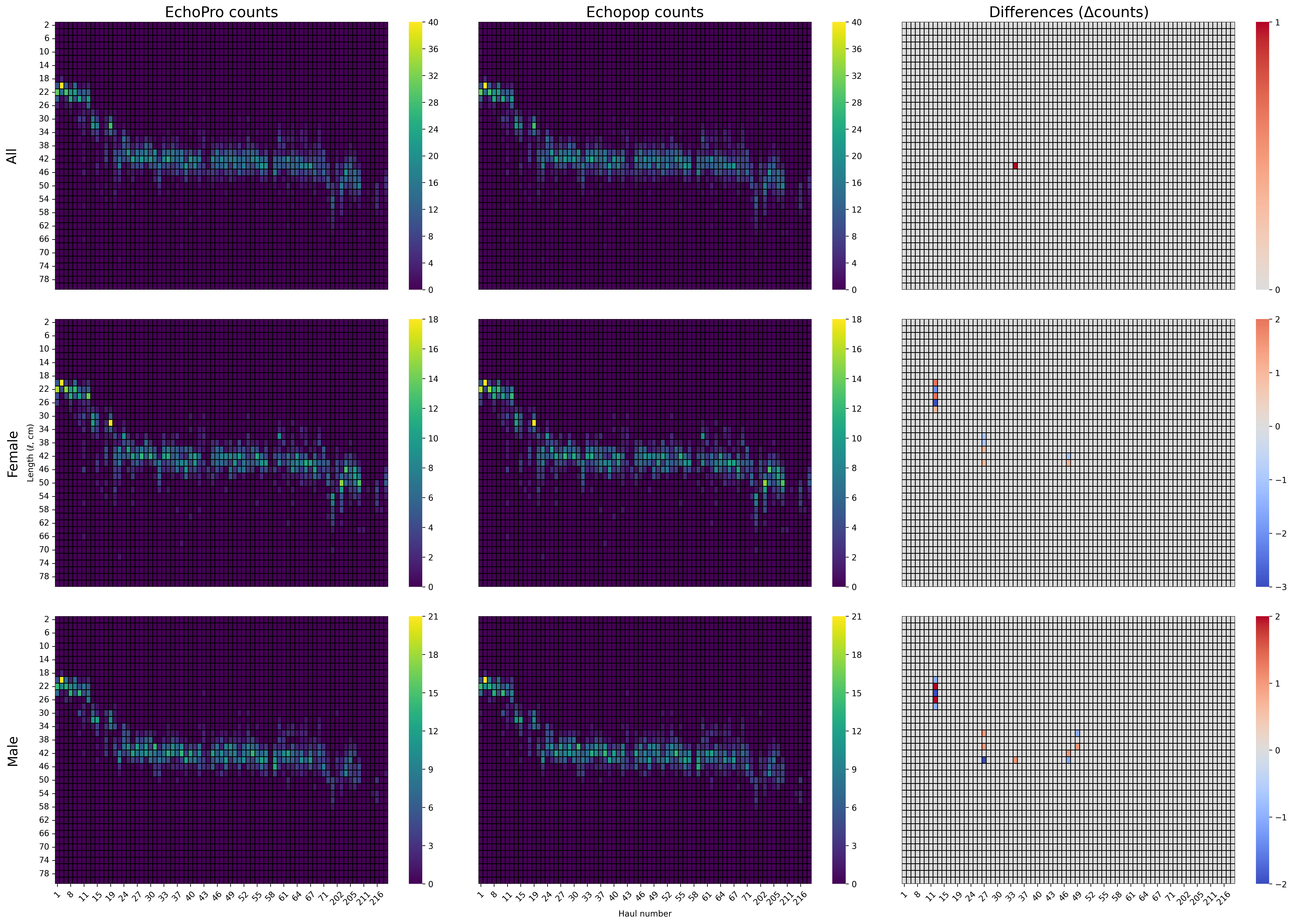
Click image to enlarge.

Total length haul counts

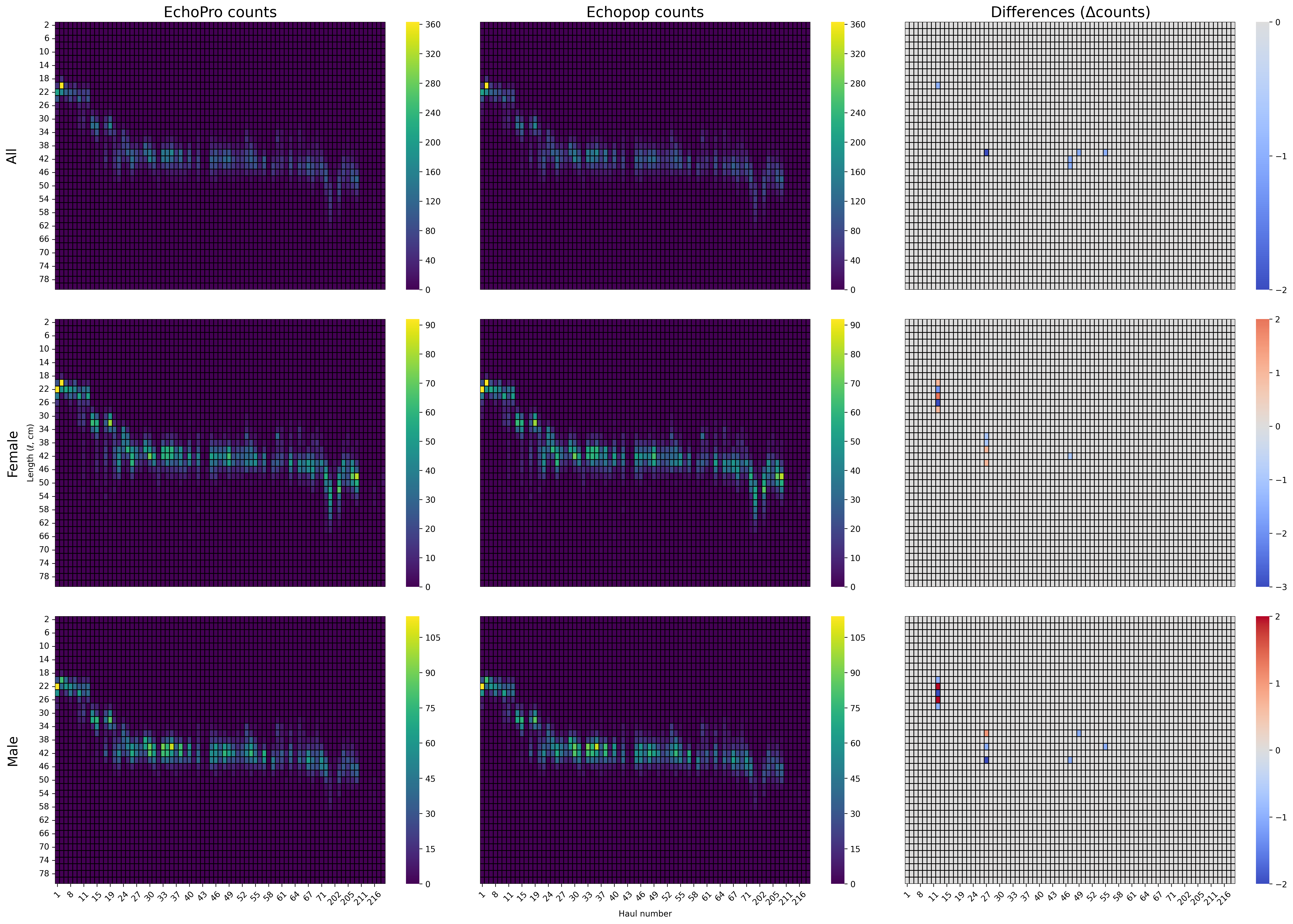
Click image to enlarge.

Length-age distributions#

The kriged reports representing the distributions of abundance and biomass over length (\(\ell\)) and age (\(\alpha\)) are ingested using the same read_pivot_table_report function as the haul-based counts.

Unlike the haul-based plot_haul_count_comparisons, these distributions are visualized via the plot_population_table_comparisons with the arguments:

echopro: The dictionary of EchoPro DataFrames.
echopop: The dictionary of Echopop DataFrames.
save_filepath: The save filepath for the resulting figure.
show_plot: The boolean flag associated with the already defined SHOW_PLOT variable. So when show_plot = False and save_filepath is parameterized, then the figure will be saved and automatically close without rendering.
log_transform: A boolean flag that when set to True log₁₀-transform the population estimates.

Otherwise, the resulting figure follows the same format as plot_haul_count_comparisons.

Kriged length-age abundance

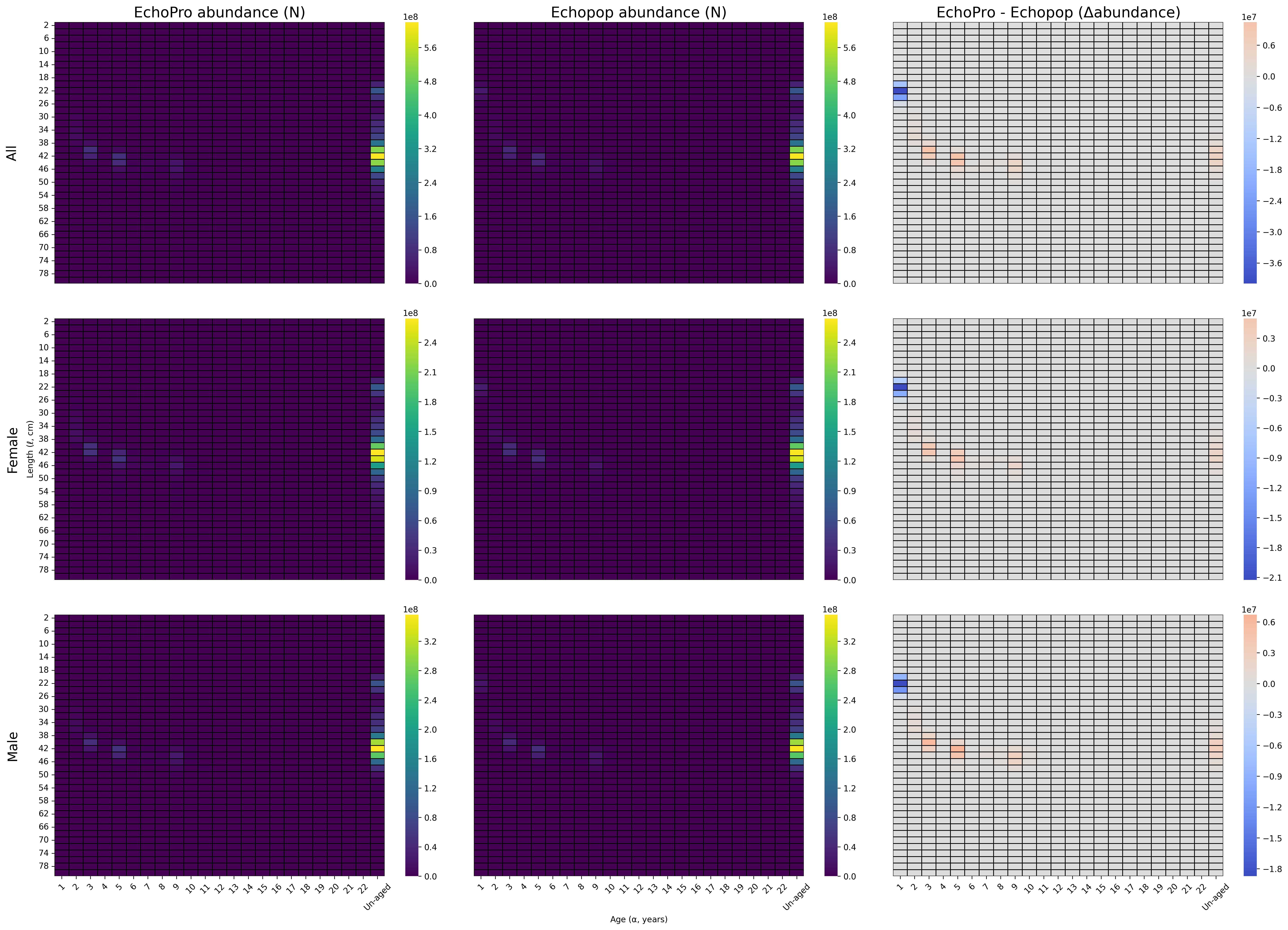
Click image to enlarge.

Kriged length-age biomass

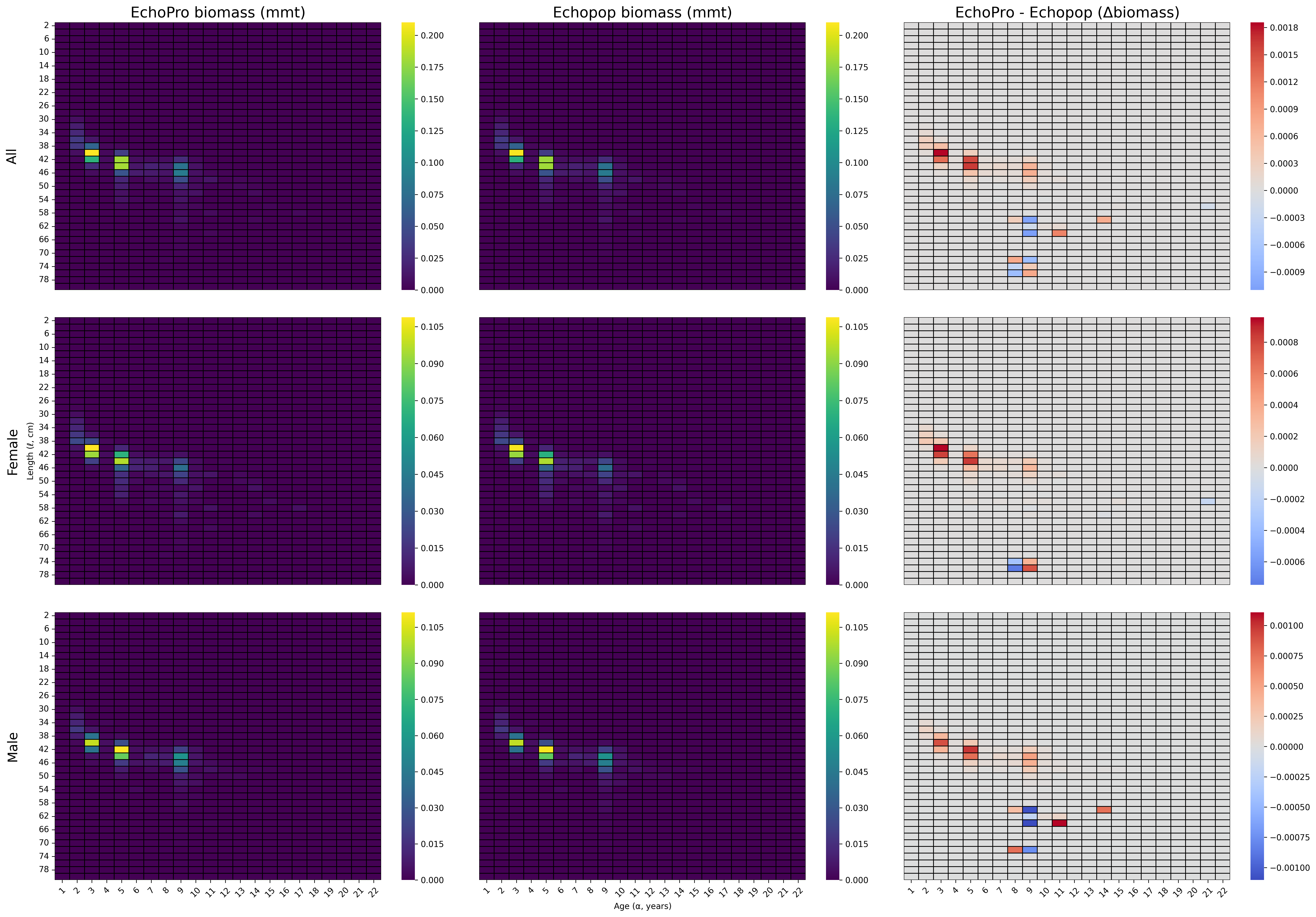
Click image to enlarge.

The same exact sequence of functions is used to produce the equivalent figures for the transect-based abundance and biomass estimates.

Transect length-age abundance

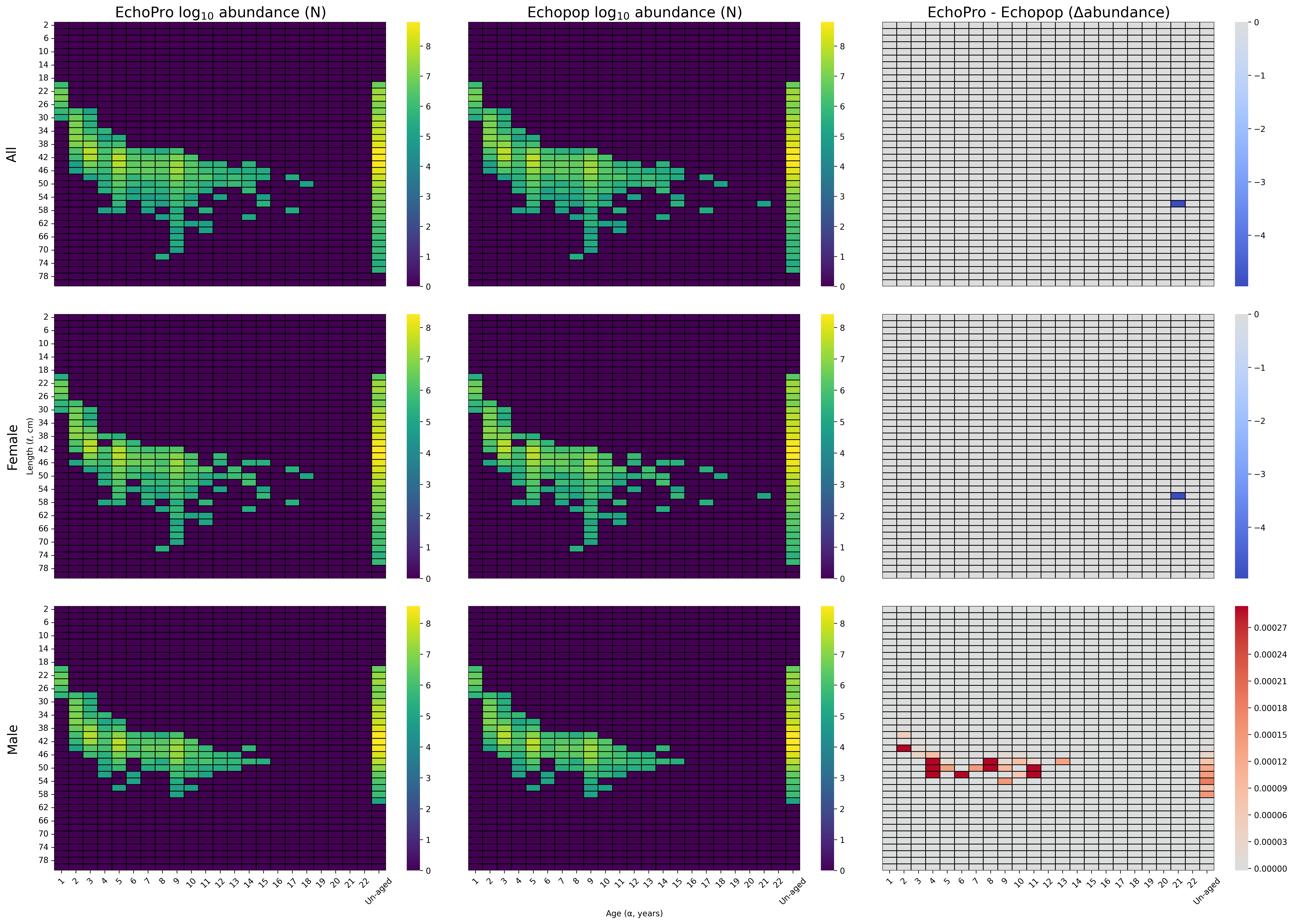
Click image to enlarge.

Transect length-age biomass

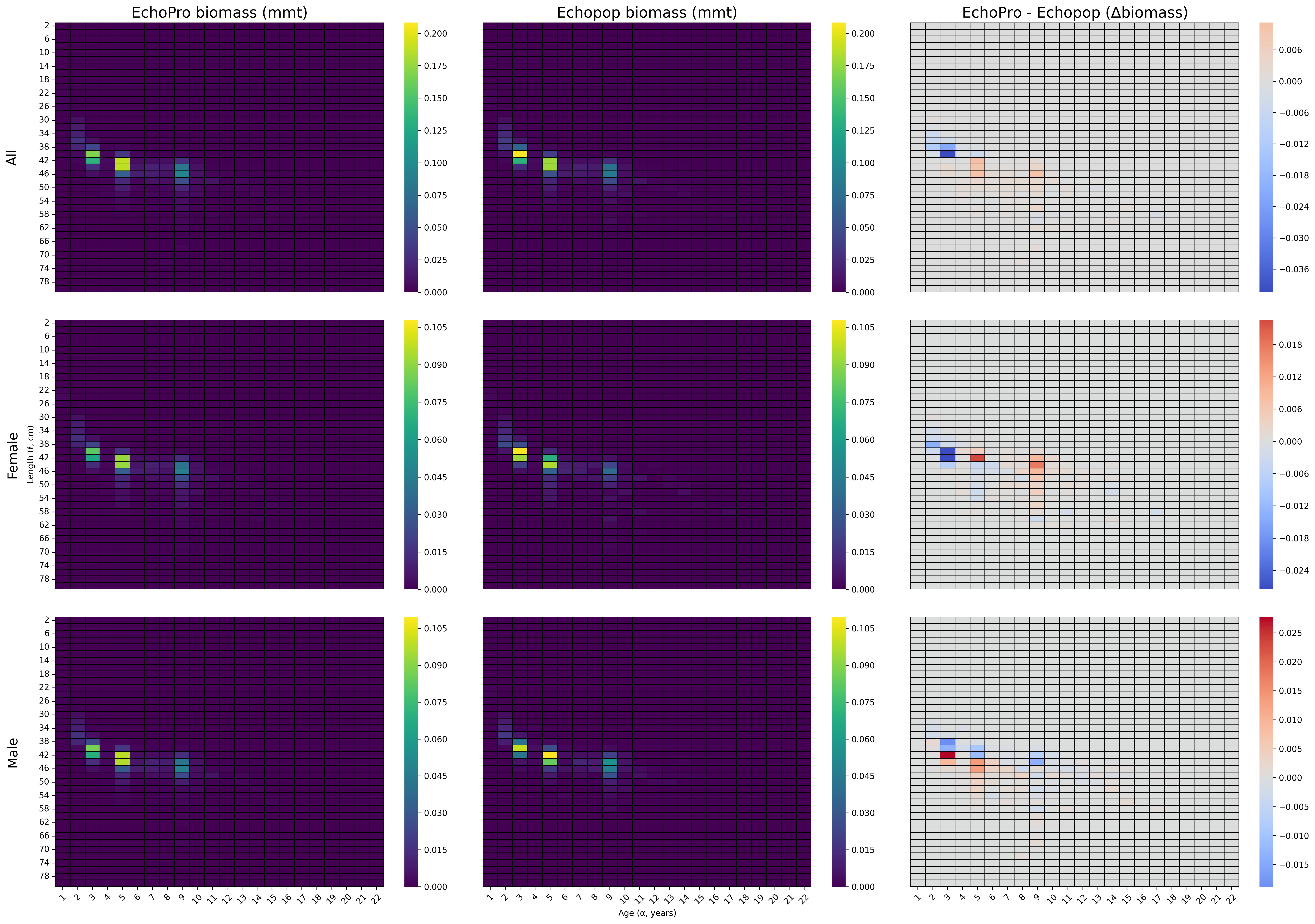
Click image to enlarge.

Spatial data#

The kriging input reports are ingested using the read_geodata function with arguments:

filepath: The filepath for the spatially distributed report.

The resulting output is a geopandas.GeoDataFrame where the coordinates are defined by the latitude and longitude of each point (using an EPSG:4326 geographic coordinate system.)

The plot_geodata function is used to plot the spatial differences between the two datasets with arguments:

echopro: The dictionary of EchoPro DataFrames.
echopop: The dictionary of Echopop DataFrames.
save_filepath: The save filepath for the resulting figure.
show_plot: The boolean flag associated with the already defined SHOW_PLOT variable. So when show_plot = False and save_filepath is parameterized, then the figure will be saved and automatically close without rendering.
log_transform: A boolean flag that when set to True log₁₀-transform the population estimates.

Although similar to the figure format as plot_haul_count_comparisons, each panel is organized slightly differently since the values from the kriging input reports are not sexed. Instead, they are organized by data variables, namely the biomass density, \(S_\text{A}\), and number density:

Variable	EchoPro	Echopop	Difference (Δquantity)
Biomass density	`[heatmap]`	`[heatmap]`	`[heatmap]`
\(S_\text{A}\)	`[heatmap]`	`[heatmap]`	`[heatmap]`
Number density	`[heatmap]`	`[heatmap]`	`[heatmap]`

Kriging input

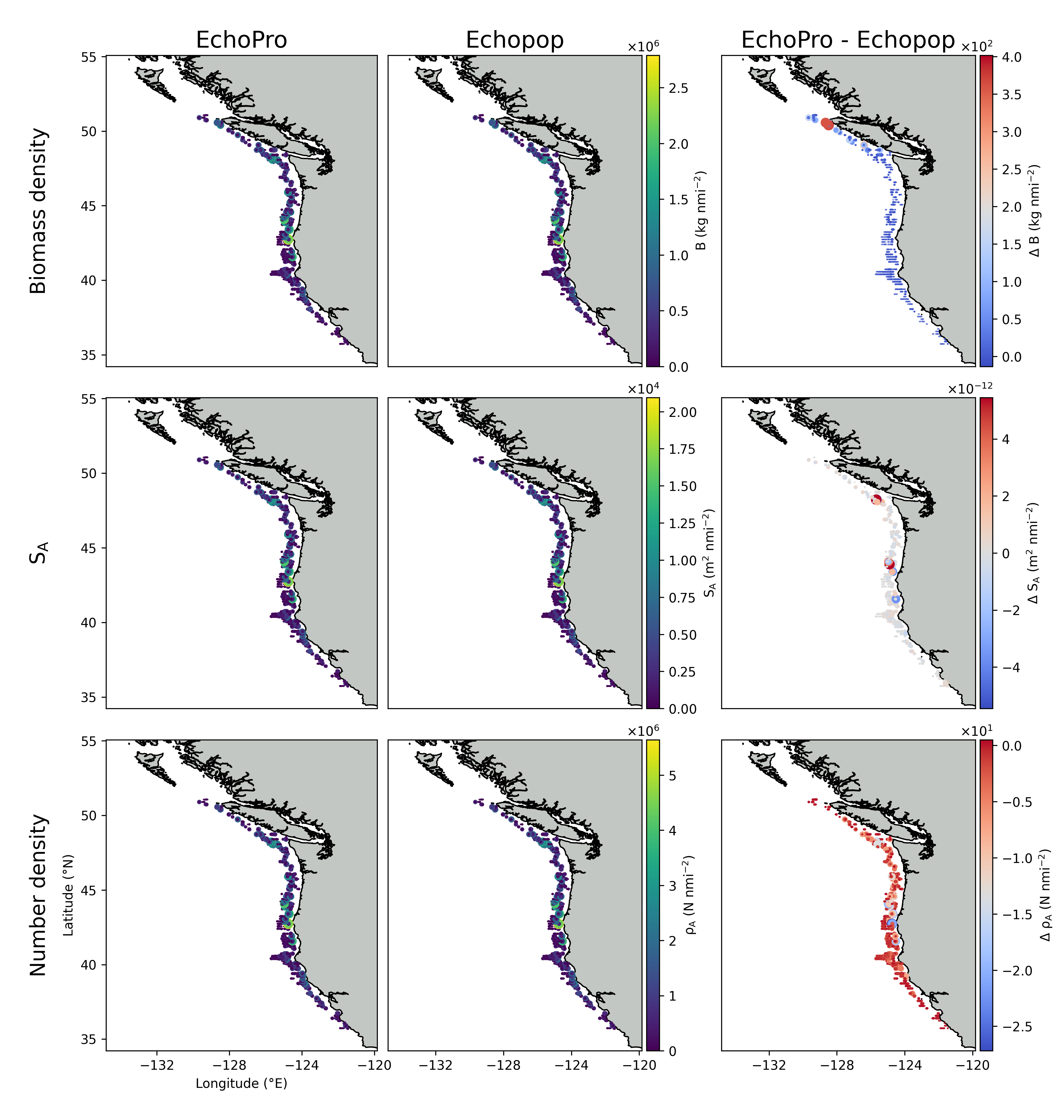
Click image to enlarge.

The transect-based population estimates are also ingested via read_geodata.

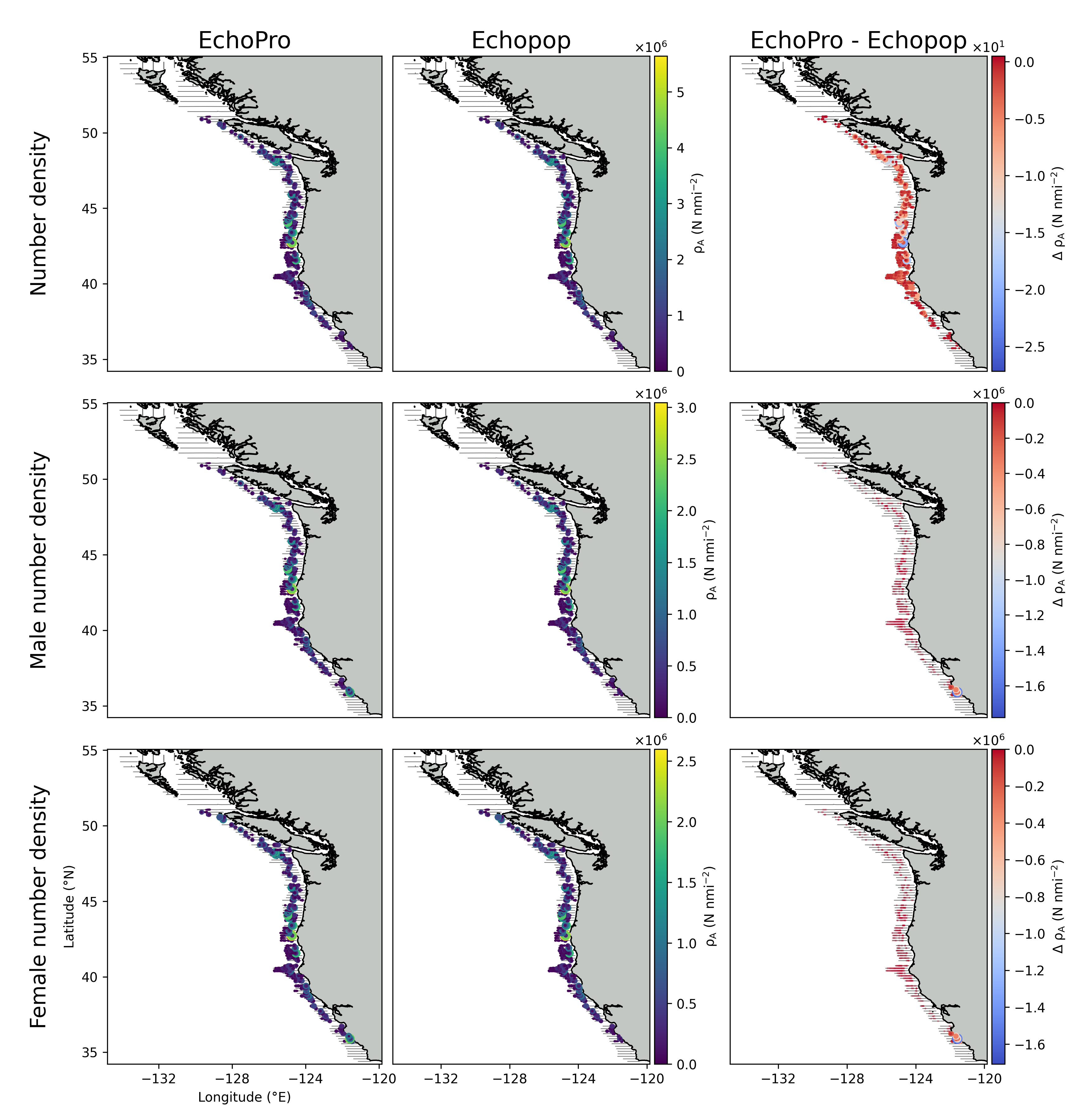
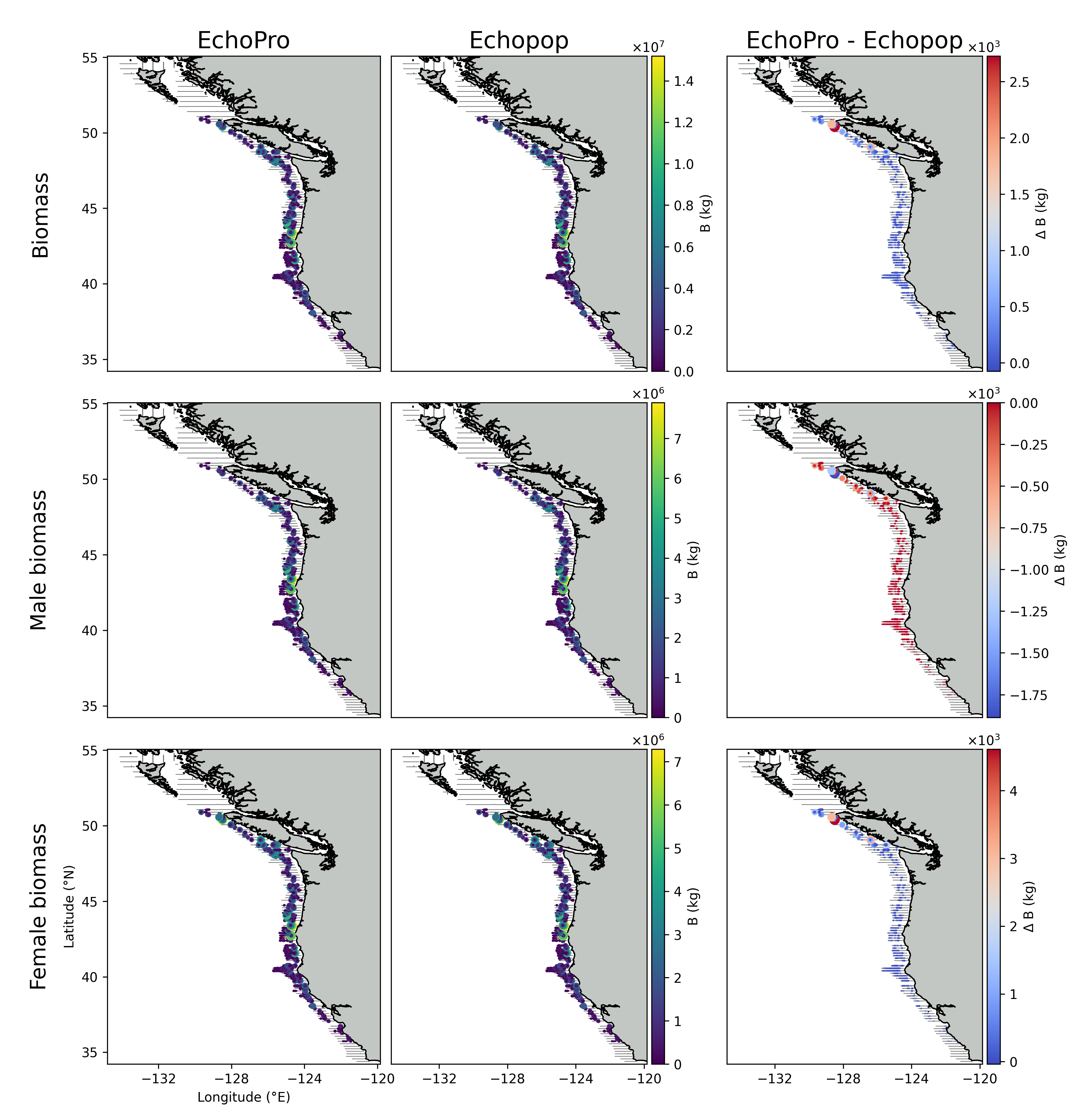
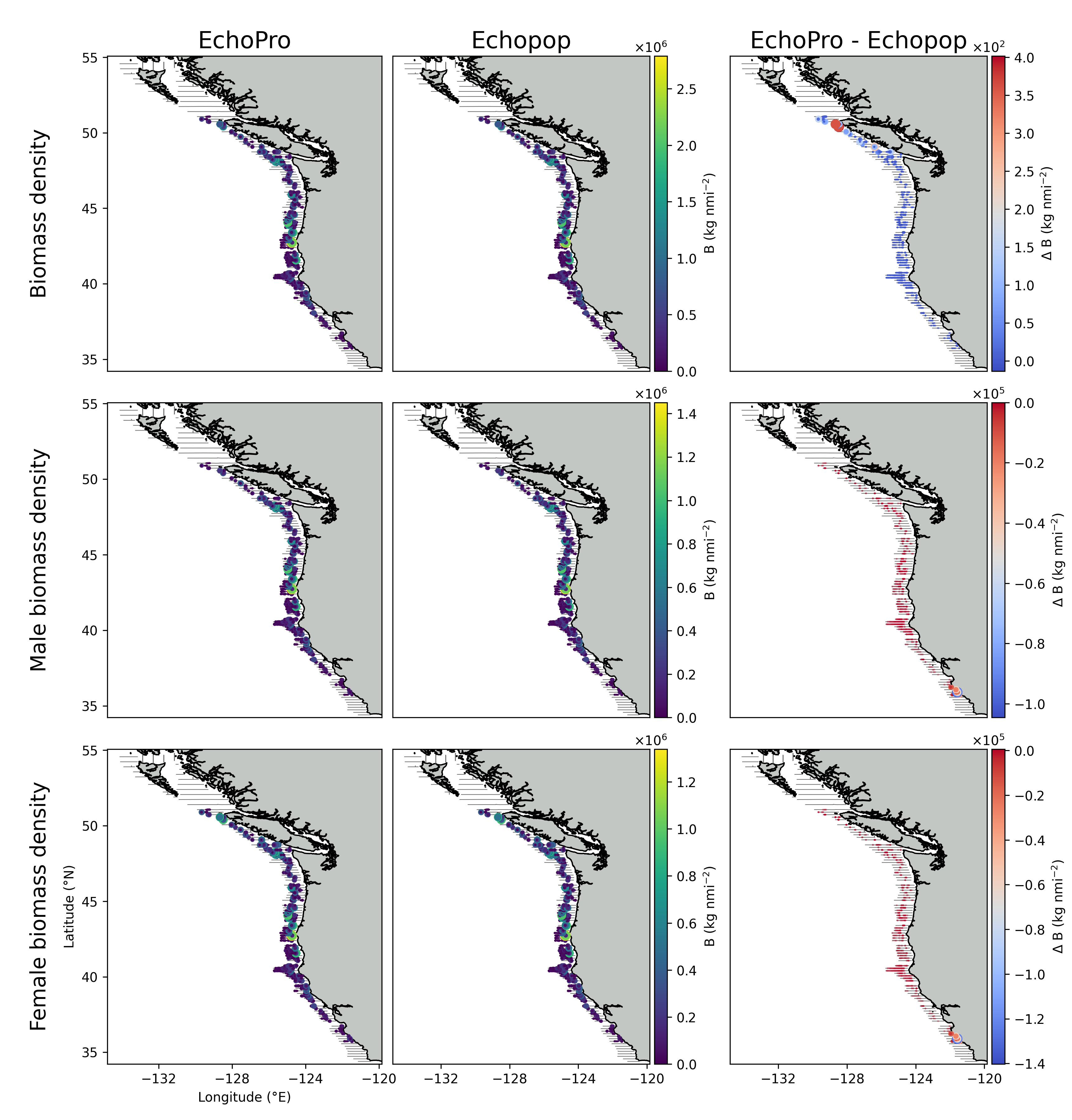
Generally speaking, plot_geodata can be applied just like it was for the kriging input report. Except unlike the kriging inputs which only comprised three variables, the population estimate reports comprise the following:

Abundances: "abundance"/"abundance_male"/"abundance_female"
Number densities: "number_density"/"number_density_male"/"number_density_female"
Biomasses: "biomass"/"biomass_male"/"biomass_female"
Biomass densities: "biomass_density"/"biomass_density_male"/"biomass_density_female"
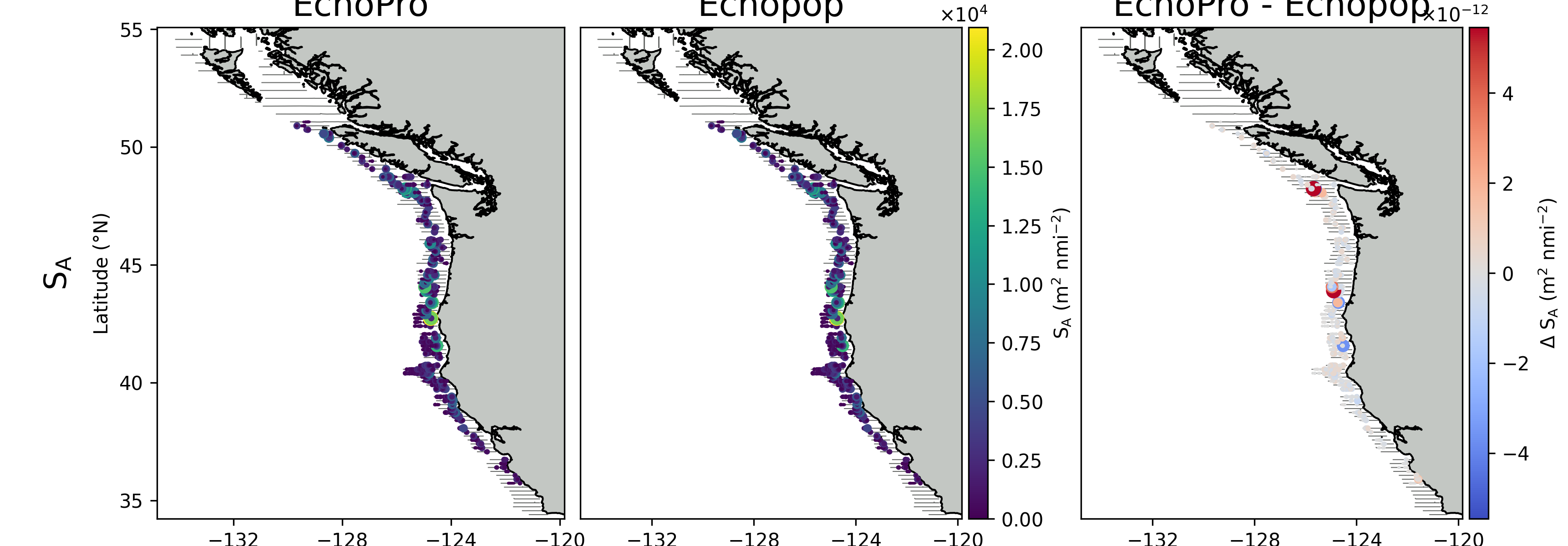
\(S_\text{A}\): "nasc"

Including all of these variables in a single figure would result in there being 13 rows, which could make the figure very difficult to interpret. The save_filepath argument for plot_geodata can either be supplied with a pathlib.Path object, or it can be supplied with a dictionary of data variable groups assigned to a single figure. For instance, if only one variable is required then:

comparisons.plot_geodata(
    ...,
    save_filepath={"nasc": SAVE_FILEPATH / "transect_nasc.png"},
    ...
)

This results in a figure with only a single row represented \(S_\text{A}\):

Variable	EchoPro	Echopop	Difference (Δquantity)
\(S_\text{A}\)	`[heatmap]`	`[heatmap]`	`[heatmap]`

If only the abundance quantities are needed, then a tuple of the desired variables for a single figure (i.e., same filepath) can be supplied:

comparisons.plot_geodata(
    ...,
    save_filepath={
        ("abundance", "abundance_male", "abundance_female"): 
            SAVE_FILEPATH / "transect_abundances.png",
        },
    ...
)

This results in a figure with three rows representing total, male, and female abundance, respectively:

Variable	EchoPro	Echopop	Difference (Δquantity)
Abundance	`[heatmap]`	`[heatmap]`	`[heatmap]`
Male abundance	`[heatmap]`	`[heatmap]`	`[heatmap]`
Female abundance	`[heatmap]`	`[heatmap]`	`[heatmap]`

Various combinations of these cases can be supplied within the same plot_geodata function call.

Transect abundances

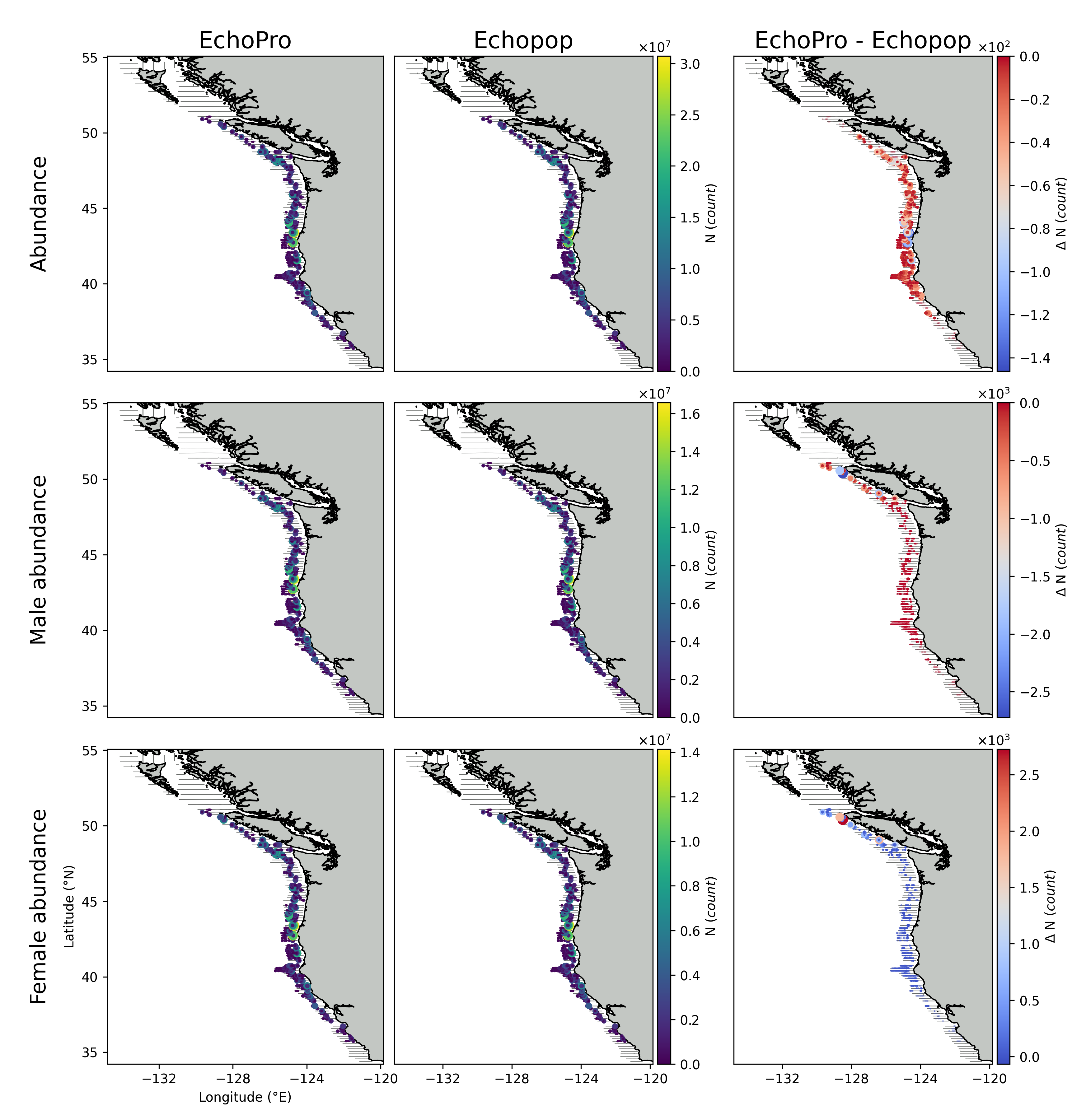
Click image to enlarge.

Transect number densities

Click image to enlarge.

Transect biomasses

Click image to enlarge.

Transect biomass densities

Click image to enlarge.

Transect NASC

Click image to enlarge.

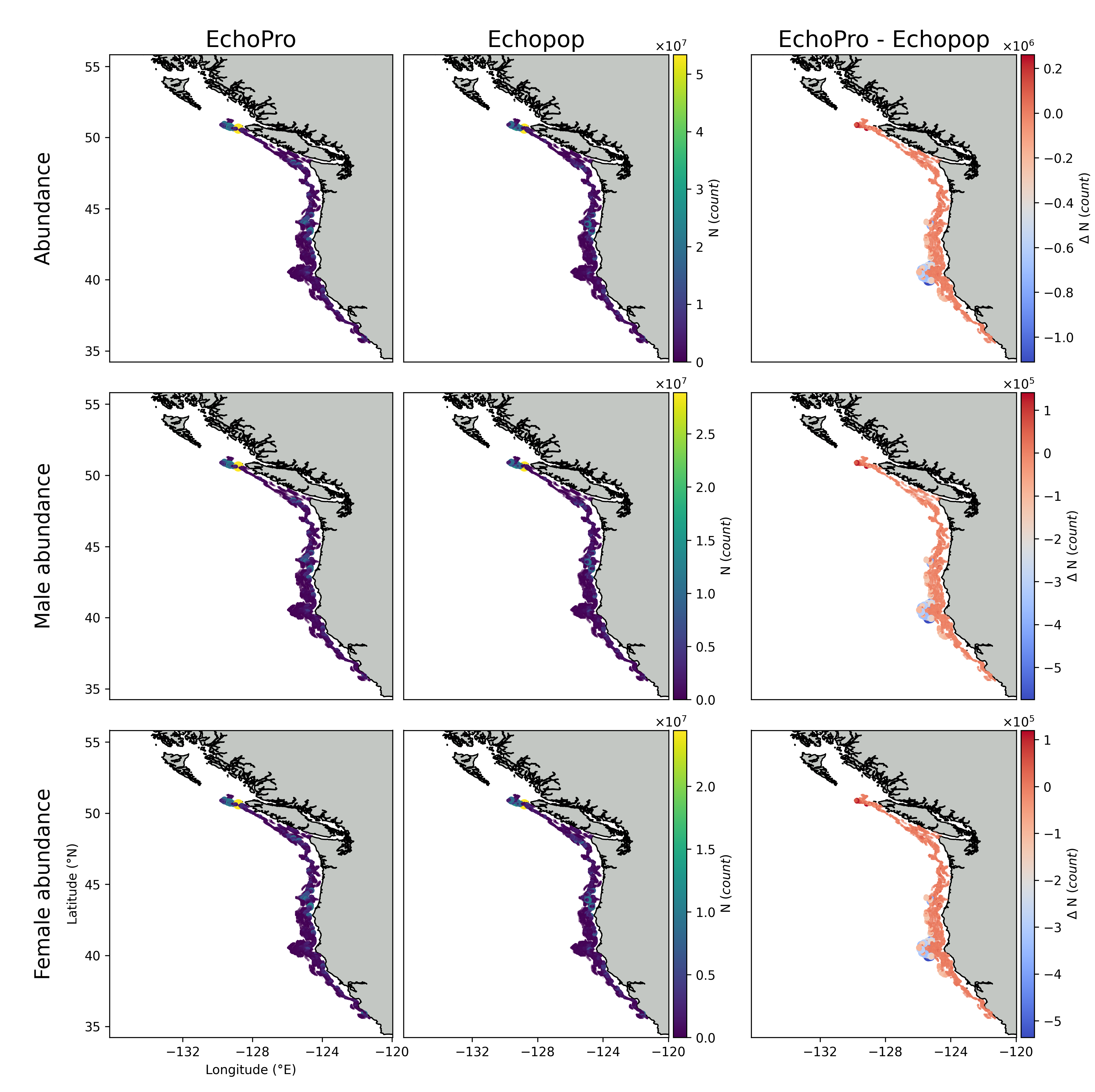
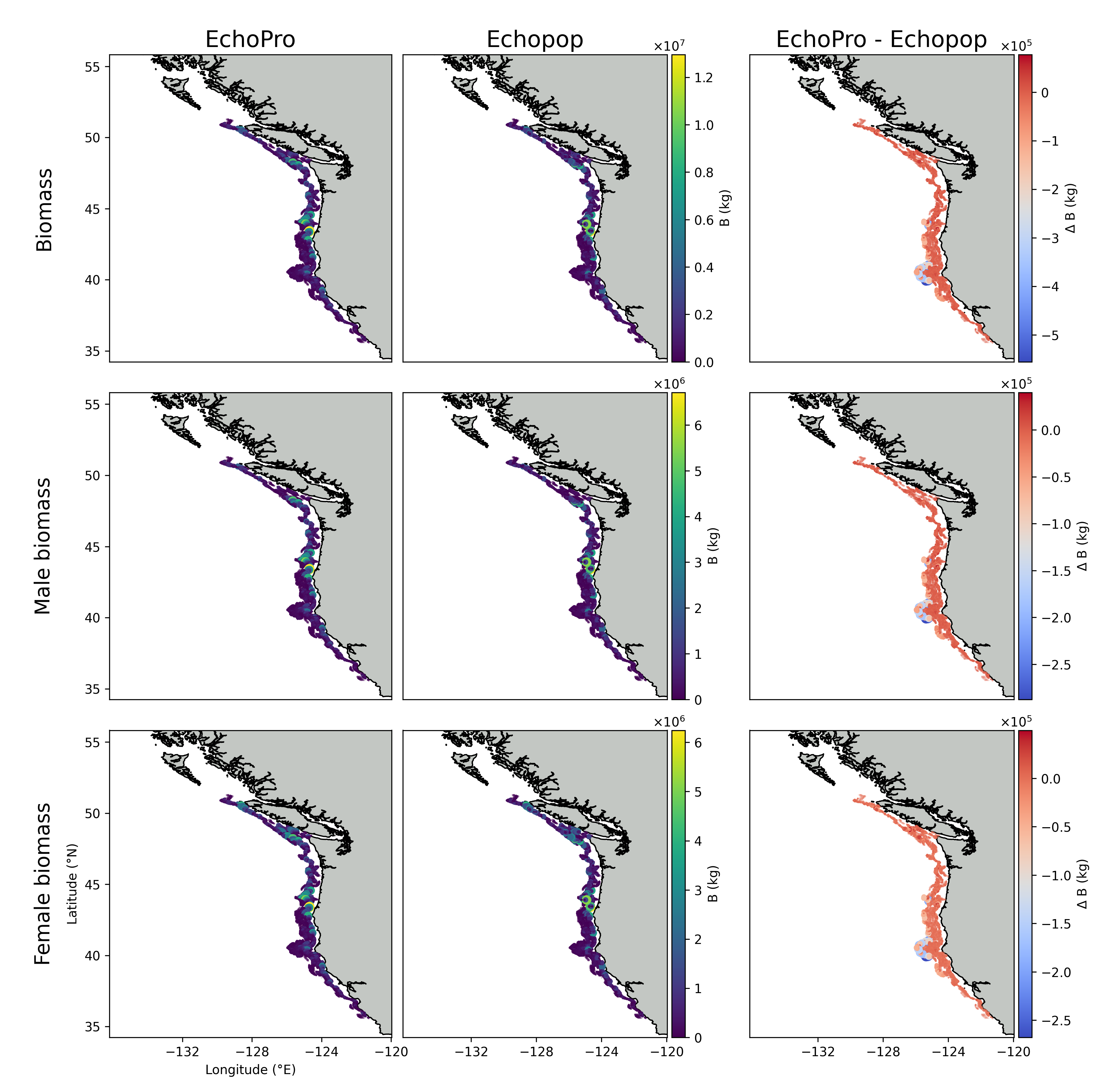
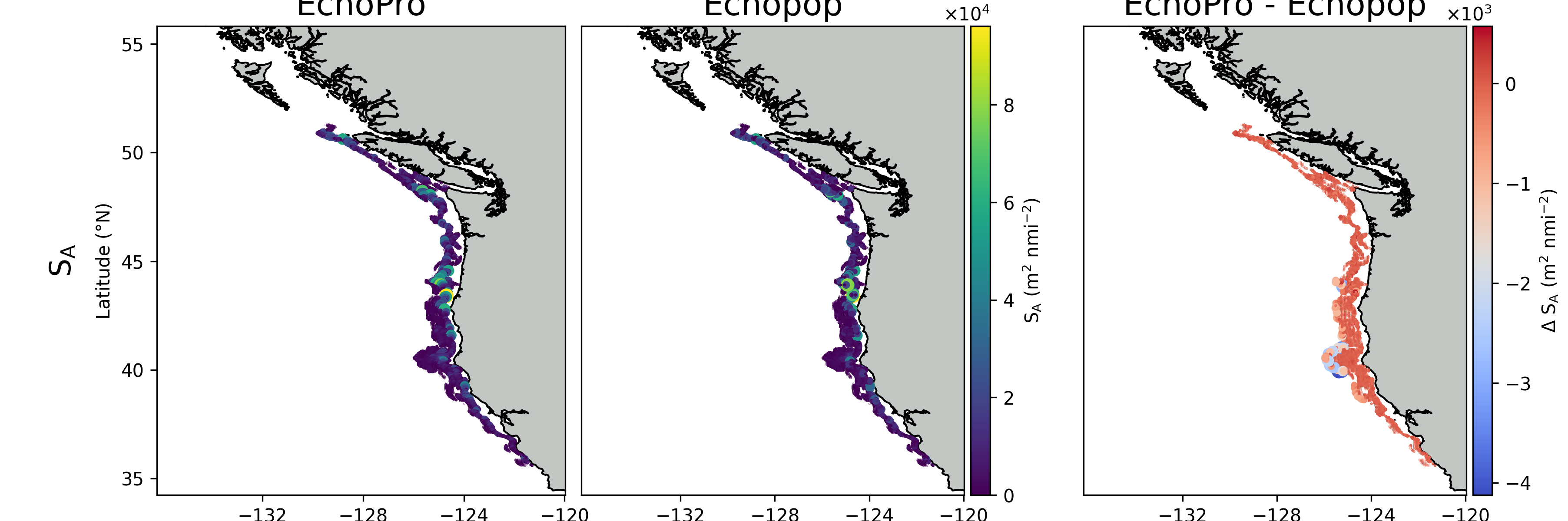
An identical sequence of function calls can be used to visualize the kriged population estimates.

Kriged abundances

Click image to enlarge.

Kriged biomasses

Click image to enlarge.

Kriged NASC

Click image to enlarge.

Making comparisons across all surveys#

Initializing ingestion#

Population estimates produced by EchoPro and Echopop can be compared across all survey years to produce a single visualization. A few variables are first defined for convenience:

SAVE_FILEPATH: The directory where all figures will be written.
YEARS: The survey years that will be processed

from datetime import date
from pathlib import Path
from typing import Callable
from echopop.reports import compare

# Set save filepath for figure
SAVE_FILEPATH = Path(
    f"C:/Data/EchopopData/cross_year_comparisons_{date.today().strftime("%Y%m%d")}.png"
)

# Survey years to process
YEARS = [1995, 1998, 2001, 2003, 2005, 2007, 2009, 2011, 2012, 2013, 2015, 2017, 2019, 2021]

Directory functions#

The ECHOPRO_ROOT and ECHOPOP_ROOT variables are lambda functions that accept a survey year and return the corresponding report directory. These can be adjusted to match any local folder structure. For example:

Flat structure with year-named subdirectories:

C:/Data/EchopopData/
└── reports/
    ├── 2019/
    │   ├── echopro/
    │   └── echopop/
    └── 2021/
        ├── echopro/
        └── echopop/

ECHOPRO_ROOT = lambda year: Path(f"C:/Data/EchopopData/reports/{year}/echopro")
ECHOPOP_ROOT = lambda year: Path(f"C:/Data/EchopopData/reports/{year}/echopop")

Per-year project folders:

C:/Data/EchopopData/
├── echopop_2019/
│   ├── reports_echopro/
│   └── reports_echopop/
└── echopop_2021/
    ├── reports_echopro/
    └── reports_echopop/

ECHOPRO_ROOT = lambda year: Path(f"C:/Data/EchopopData/echopop_{year}/reports_echopro")
ECHOPOP_ROOT = lambda year: Path(f"C:/Data/EchopopData/echopop_{year}/reports_echopop")

All reports in a single flat directory:

C:/Data/EchopopData/
└── reports/
    ├── echopro_2019/
    ├── echopop_2019/
    ├── echopro_2021/
    └── echopop_2021/

ECHOPRO_ROOT = lambda year: Path(f"C:/Data/EchopopData/reports/echopro_{year}")
ECHOPOP_ROOT = lambda year: Path(f"C:/Data/EchopopData/reports/echopop_{year}")

Filename patterns#

ECHOPOP_PATTERNS and ECHOPRO_PATTERNS are dictionaries that map each report type ("transect" and "kriging") to a filename pattern used to locate the corresponding file within each year’s report directory. Patterns can be either an exact filename string or a regex pattern — but each pattern must match exactly one file per directory.

Exact filename match — use when filenames are consistent across all years:

ECHOPOP_PATTERNS = {
    "transect": "transect_population_results_full.xlsx",
    "kriging":  "kriged_biomass_mesh_full.xlsx",
}

Regex match — use when filenames contain variable components (e.g. dates or version tags):

reports/echopro/
├── EchoPro_kriged_output-28-Jan-2026_0.xlsx   ← 2019
├── EchoPro_kriged_output-15-Mar-2024_0.xlsx   ← 2021
└── EchoPro_kriged_output-02-Feb-2023_0.xlsx   ← 2023

ECHOPRO_PATTERNS = {
    "transect": r"^EchoPro_un-kriged_output(?:-.*)?_0\.xlsx$",
    "kriging":  r"^EchoPro_kriged_output(?:-.*)?_0\.xlsx$",
}

The (?:-.*) portion matches any date or tag between the base name and the trailing _0, making the pattern robust to filename changes across survey years.

Caching and parallelization#

Two optional settings control how files are loaded across years.

CACHE_DIR specifies a directory where loaded geopandas.GeoDataFrame objects are saved as compressed cache files after their first read. On subsequent runs, cached files are loaded directly instead of re-reading the source Excel files. As more years are ingested simultaneously, caching can be significantly faster.

CACHE_DIR = Path("C:/Data/EchopopData/.cache")  # enable caching
CACHE_DIR = None                                # disable caching

This is most useful when iterating on the comparison plots without changing the underlying data, e.g., adjusting figure aesthetics or testing different year subsets.

MAX_WORKERS controls whether files are loaded sequentially or in parallel using a thread pool.

MAX_WORKERS = None  # sequential (default, safest across all OS)
MAX_WORKERS = 8     # parallel with 8 threads

Sequential loading (None) is the safest default and is recommended when:

Running on Windows, where thread safety with file I/O can be unpredictable
Debugging load errors, since parallel exceptions can be harder to trace

Parallel loading is useful when:

Loading a large number of years (e.g. all 14 survey years)
The source files are on a fast local disk or SSD
You are confident the files and directories are all present and well-formed

A value of 4–8 is typically sufficient. Beyond that, disk I/O rather than CPU becomes the bottleneck.

Data ingestion#

All georeferenced population estimate reports are loaded in a single call to load_all_geodata_reports with arguments:

years: A list of survey years to load (e.g. [2019, 2021]).
echopro_root: A callable that accepts a year and returns the EchoPro report directory.
echopop_root: A callable that accepts a year and returns the Echopop report directory.
echopro_patterns: A dictionary mapping report type to an EchoPro filename pattern.
echopop_patterns: A dictionary mapping report type to an Echopop filename pattern.
cache_dir: An optional directory for caching loaded GeoDataFrame objects. Set to None to disable.
max_workers: An optional integer controlling parallel loading. Set to None for sequential loading.
verbose: If True, prints each file path as it is loaded. Useful for debugging or monitoring progress across many years.

This returns two nested dictionaries, one for EchoPro and one for Echopop, each organized by report type and year:

ECHOPRO_DATASETS = {
    "transect": {1995: GeoDataFrame, 1998: GeoDataFrame, ..., 2021: GeoDataFrame},
    "kriging":  {1995: GeoDataFrame, 1998: GeoDataFrame, ..., 2021: GeoDataFrame},
}

Each geopandas.GeoDataFrame contains the georeferenced population estimates for a single survey year and report type, with columns for abundance, biomass, nasc, and associated spatial coordinates. Any years or files that fail to load are skipped with a printed error message rather than raising an exception, allowing the remaining years to continue loading.

Computing differences#

Once all reports are loaded, the total population estimates are compared across years and report types using compute_dataset_differences with the arguments:

echopro_datasets: The nested dictionary of EchoPro GeoDataFrame objects returned by load_all_geodata_reports.
echopop_datasets: The nested dictionary of Echopop GeoDataFrame objects returned by load_all_geodata_reports.
columns: The columns to sum and compare. Defaults to ["abundance", "biomass", "nasc"].

This returns two pandas.DataFrame objects, both indexed by (report_type, year):

magnitude_differences: The raw magnitude difference (EchoPro - Echopop) for each column, year, and report type.
percent_differences: The signed percent difference relative to the mean of both datasets, i.e.:

\[ \%\text{Difference} = \frac{ \text{X}_\text{Echopop} - \text{X}_\text{EchoPro} }{ \text{X}_\text{EchoPro} } \times 100, \]

where \(\text{X}\) is a specific quantity, such as NASC, biomass density, biomass, etc. Positive values indicate EchoPro exceeds Echopop; negative values indicate the opposite.

Visualizing the differences#

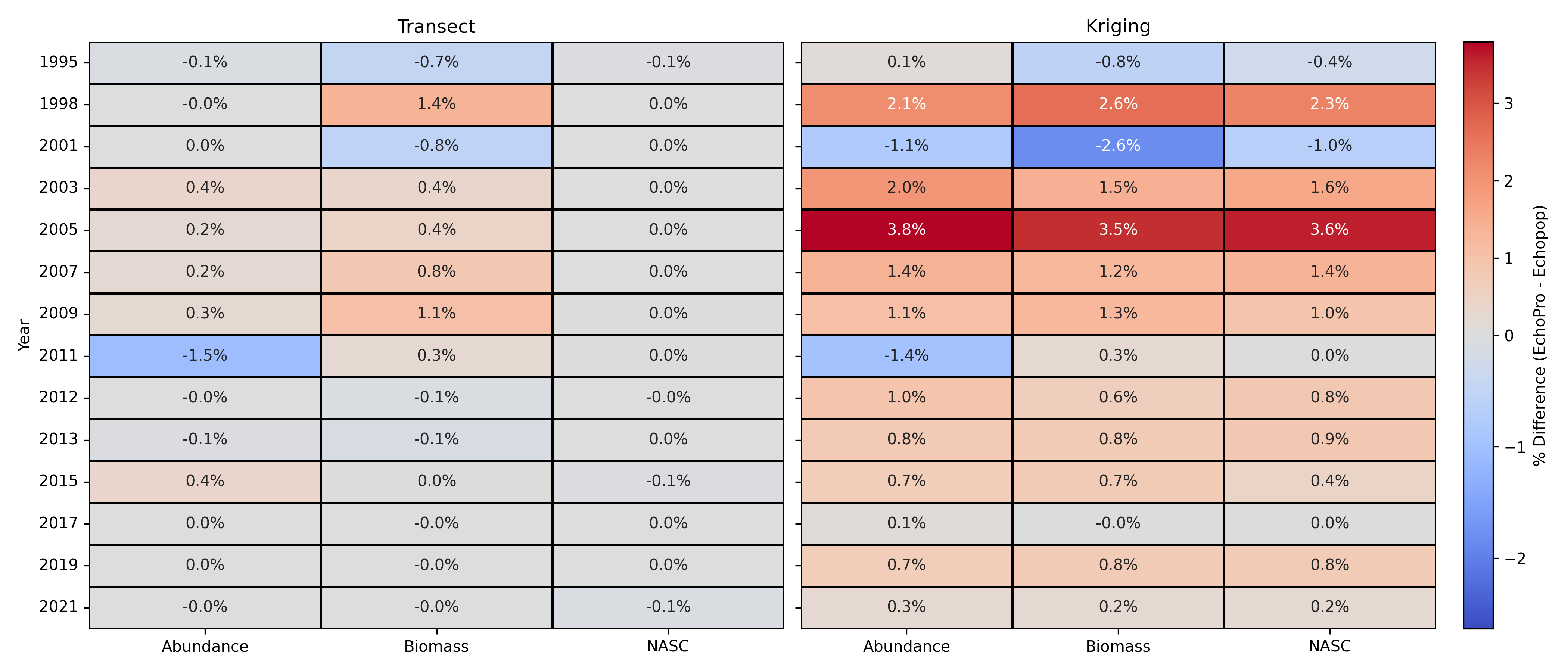
The signed percent differences are visualized across all survey years and report types using plot_dataset_differences with arguments:

signed_percent_differences: The signed percent differences returned by compute_dataset_differences.
save_filepath: The filepath for the resulting figure. Set to None to only display without saving.
columns: The columns to display on the x-axis. Defaults to ["abundance", "biomass", "nasc"].
figsize: The figure size in inches. Defaults to (14, 6).

This produces a two-panel heatmap figure, one panel per report type ("transect" and "kriging"), where each cell displays the signed percent difference for a given year and quantity:

Year	Transect abundance	Transect biomass	Transect S_A	Kriged abundance	Kriged biomass	Kriged S_A
1995	`[%diff]`	`[%diff]`	`[%diff]`	`[%diff]`	`[%diff]`	`[%diff]`
1998	`[%diff]`	`[%diff]`	`[%diff]`	`[%diff]`	`[%diff]`	`[%diff]`
⋮	⋮	⋮	⋮	⋮	⋮	⋮
2021	`[%diff]`	`[%diff]`	`[%diff]`	`[%diff]`	`[%diff]`	`[%diff]`

Positive values (red) indicate EchoPro exceeds Echopop; negative values (blue) indicate the opposite. A single shared colorbar is placed to the right of both panels.

Cross-year comparisons

Click image to enlarge.

Compare EchoPro and Echopop reports

Contents

Compare EchoPro and Echopop reports#

Visualizing year-specific differences#

Haul-based reports#

Length-age distributions#

Spatial data#

Making comparisons across all surveys#

Initializing ingestion#

Directory functions#

Filename patterns#

Caching and parallelization#

Data ingestion#

Computing differences#

Visualizing the differences#