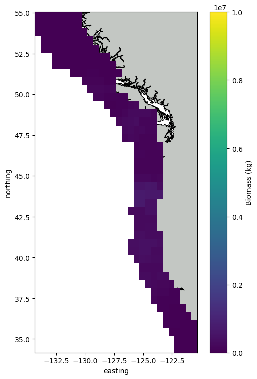
Plot results

A variety of plots can be generated using the graphics module. These include the following types:

• plot_age_length_heatmap: Plotting the age-length heatmap of abundance, biomass, etc.

• plot_kriged_mesh: Plotting the kriged mesh or survey data using several methods.

• plot_transect_map: Plotting the survey transects and variables on a map.

Plotting function keyword arguments

All plotting functions allow for matplotlib.pyplot-specific keyword arguments, such as for imshow, scatter, etc.

Import necessary modules

The module can be imported directly from Echopop.

from echopop import graphics as egra

A save directory can be optionally set that will generate the figures at the defined filepath.

SAVE_DIRECTORY = Path("C:/Data/Figures")

Age-length heatmap

Distributions of abundance and biomass along length and age for each sex can be visualized via plot_age_length_heatmap. This expects the input table to be a multiindex table. This requires columns to be indexed by (age_bin, sex), and for rows to be indexed by length_bin. When examining the appropriate input xarray.DataArray, it should resemble the following:

<xarray.DataArray 'biomass' (length_bin: 40, sex: 2, age_bin: 22)> Size: 14kB
array([[[  0.        ,   0.        ,   0.        , ...,   0.        ,
           0.        ,   0.        ],
        [  0.        ,   0.        ,   0.        , ...,   0.        ,
           0.        ,   0.        ]],

       [[  0.        ,   0.        ,   0.        , ...,   0.        ,
           0.        ,   0.        ],
        [  0.        ,   0.        ,   0.        , ...,   0.        ,
           0.        ,   0.        ]],

       [[353.63810194,   0.        ,   0.        , ...,   0.        ,
           0.        ,   0.        ],
        [269.5325609 ,   0.        ,   0.        , ...,   0.        ,
           0.        ,   0.        ]],

       ...,

       [[  0.        ,   0.        ,   0.        , ...,   0.        ,
           0.        ,   0.        ],
        [  0.        ,   0.        ,   0.        , ...,   0.        ,
           0.        ,   0.        ]],

       [[  0.        ,   0.        ,   0.        , ...,   0.        ,
           0.        ,   0.        ],
        [  0.        ,   0.        ,   0.        , ...,   0.        ,
           0.        ,   0.        ]],

       [[  0.        ,   0.        ,   0.        , ...,   0.        ,
           0.        ,   0.        ],
        [  0.        ,   0.        ,   0.        , ...,   0.        ,
           0.        ,   0.        ]]], shape=(40, 2, 22))
Coordinates:
  * length_bin  (length_bin) category 680B (1.0, 3.0] ... (79.0, 81.0]
  * sex         (sex) object 16B 'female' 'male'
  * age_bin     (age_bin) category 374B (0.5, 1.5] (1.5, 2.5] ... (21.5, 22.5]

xarray.DataArray

'biomass'

• length_bin: 40
• sex: 2
• age_bin: 22

• 0.0 0.0 0.0 0.0 0.0 0.0 0.0 0.0 ... 0.0 0.0 0.0 0.0 0.0 0.0 0.0 0.0

  array([[[  0.        ,   0.        ,   0.        , ...,   0.        ,
             0.        ,   0.        ],
          [  0.        ,   0.        ,   0.        , ...,   0.        ,
             0.        ,   0.        ]],
  
         [[  0.        ,   0.        ,   0.        , ...,   0.        ,
             0.        ,   0.        ],
          [  0.        ,   0.        ,   0.        , ...,   0.        ,
             0.        ,   0.        ]],
  
         [[353.63810194,   0.        ,   0.        , ...,   0.        ,
             0.        ,   0.        ],
          [269.5325609 ,   0.        ,   0.        , ...,   0.        ,
             0.        ,   0.        ]],
  
         ...,
  
         [[  0.        ,   0.        ,   0.        , ...,   0.        ,
             0.        ,   0.        ],
          [  0.        ,   0.        ,   0.        , ...,   0.        ,
             0.        ,   0.        ]],
  
         [[  0.        ,   0.        ,   0.        , ...,   0.        ,
             0.        ,   0.        ],
          [  0.        ,   0.        ,   0.        , ...,   0.        ,
             0.        ,   0.        ]],
  
         [[  0.        ,   0.        ,   0.        , ...,   0.        ,
             0.        ,   0.        ],
          [  0.        ,   0.        ,   0.        , ...,   0.        ,
             0.        ,   0.        ]]], shape=(40, 2, 22))

• Coordinates: (3)
  • length_bin
    (length_bin)
    category
    (1.0, 3.0] ... (79.0, 81.0]

    [(1.0, 3.0], (3.0, 5.0], (5.0, 7.0], (7.0, 9.0], (9.0, 11.0], ..., (71.0, 73.0], (73.0, 75.0], (75.0, 77.0], (77.0, 79.0], (79.0, 81.0]]
    Length: 40
    Categories (40, interval[float64, right]): [(1.0, 3.0] < (3.0, 5.0] < (5.0, 7.0] < (7.0, 9.0] ... (73.0, 75.0] < (75.0, 77.0] < (77.0, 79.0] < (79.0, 81.0]]

  • sex
    (sex)
    object
    'female' 'male'

    array(['female', 'male'], dtype=object)

  • age_bin
    (age_bin)
    category
    (0.5, 1.5] ... (21.5, 22.5]

    [(0.5, 1.5], (1.5, 2.5], (2.5, 3.5], (3.5, 4.5], (4.5, 5.5], ..., (17.5, 18.5], (18.5, 19.5], (19.5, 20.5], (20.5, 21.5], (21.5, 22.5]]
    Length: 22
    Categories (22, interval[float64, right]): [(0.5, 1.5] < (1.5, 2.5] < (2.5, 3.5] < (3.5, 4.5] ... (18.5, 19.5] < (19.5, 20.5] < (20.5, 21.5] < (21.5, 22.5]]

The plot_age_length_heatmap function has many arguments that can configure the table to one’s preferences.

• data: The input xarrayDataArray with the coordinates "length_bin" and "age_bin".

• include_filter: Optional dictionary of filters to include specific data.

• exclude_filter: Optional dictionary of filters to exclude specific data.

• replace_value: Values excluded by exclude_filter can be optionally replaced with a set value (e.g. 0.0) instead of being completely removed.

• axis_kwargs: Keyword arguments for axis formatting (e.g. labels) used by matplotlib.pyplot.

• plot_kwargs: Keyword arguments used by matplotliib.pyplot.subplots.

• colorbar_kwargs: Keyword arguments for matplotlib.pyplot.colorbar.

• imshow_kwargs: Keyword arguments for matplotlib.axes.Axes.imshow.

• save_path: A pathlib.Path object defining the filepath for where the figure should be saved.

• savefig_kwargs: Keyword arguments for matplotlib.pyplot.savefig.

Basic plotting

The most basic version of this plot can be generated via:

egra.plot_age_length_heatmap(data=da_kriged_biomass_table)

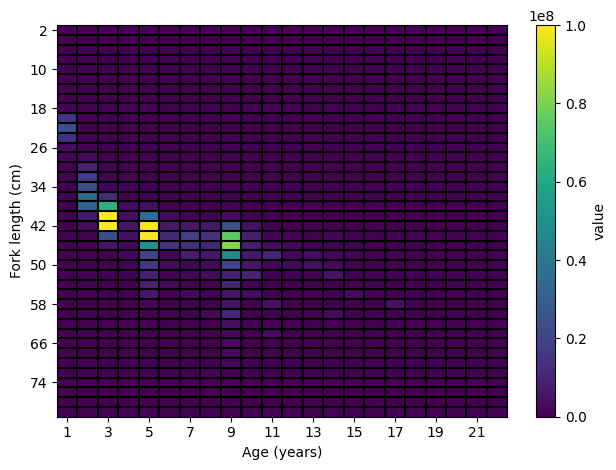
Here, all counts for each age-length cell have been summed, which means that this figure represents the combined male and female contributes to the kriged biomass estimates. Because we typically want descriptive labels, we can amend the figure using some of the matplotlib.pyplot keyword arguments:

egra.plot_age_length_heatmap(
    data=da_kriged_biomass_table,
    colorbar_kwargs={"label": "Combined biomass (male+female, kg)"},
    axis_kwargs={"ylabel": r"Fork length ($\mathregular{\ell}$, cm)", 
                 "xlabel": r"Otolith age ($\mathregular{\alpha}$, years)"},
)

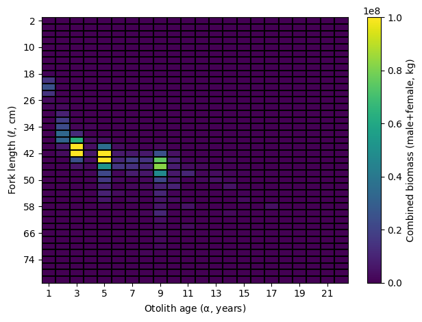
To save the figure, we can then add the savepath and optional savefig_kwargs:

egra.plot_age_length_heatmap(
    data=da_kriged_biomass_table,
    colorbar_kwargs={"label": "Combined biomass (male+female, kg)"},
    axis_kwargs={"ylabel": r"Fork length ($\mathregular{\ell}$, cm)", 
                 "xlabel": r"Otolith age ($\mathregular{\alpha}$, years)"},
    savepath=SAVE_DIRECTORY / "kriged_biomass_age_length_heatmap_plus.png",
    savefig_kwargs={"dpi": 300},
)

Filtering by age and sex

The age-length heatmap can be refined for specific sexes, lengths, and ages by using the include_filter, exclude_filter, and replace_value arguments. For instance, the male-only figure can be generated via:

egra.plot_age_length_heatmap(
    data=da_kriged_biomass_table,
    include_filter={"sex": "male"},
    colorbar_kwargs={"label": "Male biomass (kg)"},
    axis_kwargs={"ylabel": r"Fork length ($\mathregular{\ell}$, cm)", 
                 "xlabel": r"Otolith age ($\mathregular{\alpha}$, years)"},
)

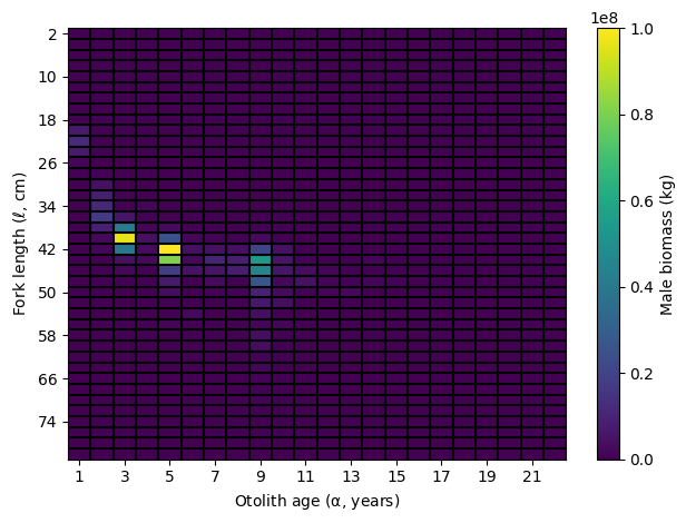
For this dataset, include_filter("sex": "male") would be equivalent to exclude_filter("sex": "female") since only male and female fish contribute to this particular table (note: this may not always be the case). Similarly, specific ages can be excised from the dataset:

egra.plot_age_length_heatmap(
    data=da_kriged_biomass_table,
    include_filter={"sex": "male"},
    exclude_filter={"age_bin": [0, 1]},
    colorbar_kwargs={"label": "Age-2+ male biomass (kg)"},
    axis_kwargs={"ylabel": r"Fork length ($\mathregular{\ell}$, cm)", 
                 "xlabel": r"Otolith age ($\mathregular{\alpha}$, years)"},
)

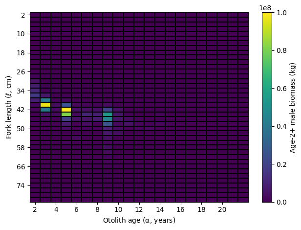
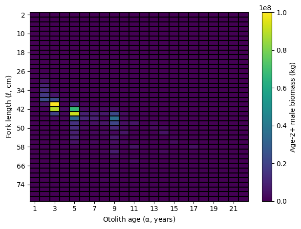
Here, all age columns less than 2 years have been completely removed. Alternatively, we may want to retain that column but simply set it to 0.0:

egra.plot_age_length_heatmap(
    data=da_kriged_biomass_table,
    include_filter={"sex": "male"},
    exclude_filter={"age_bin": [0, 1]},
    replace_value=0.0,
    colorbar_kwargs={"label": "Age-2+ male biomass (kg)"},
    axis_kwargs={"ylabel": r"Fork length ($\mathregular{\ell}$, cm)", 
                 "xlabel": r"Otolith age ($\mathregular{\alpha}$, years)"},
)

Adjusting the aesthetics

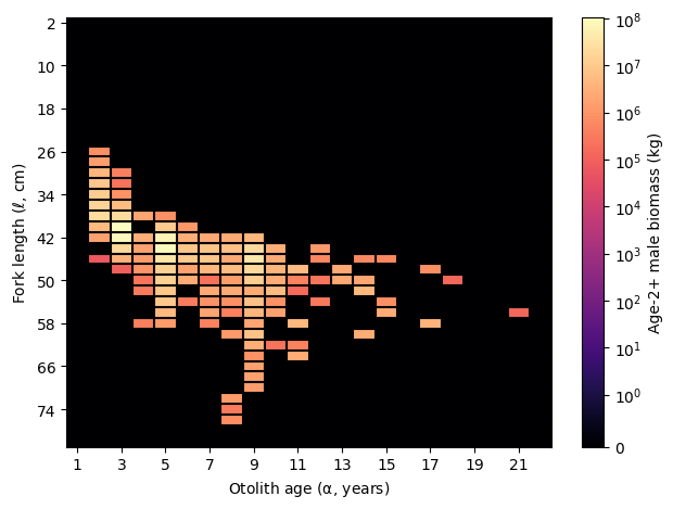
The skew of these distributions can obscure the colormap. Both colorbar_kwargs and imshow_kwargs can be adjusted to help “even” out or adjust the aesthetics of the plot to make the smaller values more prominent and separated from the background values of 0.0. First, we can create an entirely new scaled colormap using log scaling:

from matplotlib.colors import SymLogNorm
import matplotlib.pyplot as plt

# Define scale 
norm = SymLogNorm(linthresh=1., vmin=0., vmax=da_kriged_biomass_table.max().max())

# Create colormap
scaled_colormap = plt.cm.ScalarMappable(norm=norm, cmap="magma")

We can then add the normalized values and corresponding scaled colormap to the plot:

egra.plot_age_length_heatmap(
    data=da_kriged_biomass_table,
    include_filter={"sex": "male"},
    exclude_filter={"age_bin": [0, 1]},
    replace_value=0.0,
    colorbar_kwargs={"mappable": scaled_colormap, "label": "Age-2+ male biomass (kg)"},
    imshow_kwargs={"norm": norm, "cmap": "magma"},
    axis_kwargs={"ylabel": r"Fork length ($\mathregular{\ell}$, cm)", 
                 "xlabel": r"Otolith age ($\mathregular{\alpha}$, years)"},
)

Transect map

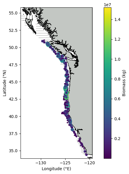
Spatial distributions of different along-transect variables can be visualized via plot_transect_map. This expects a pandas.DataFrame or geopandas.GeoDataFrame comprising appropriate coordinates (e.g. longitude, latitude). The plot_transect_map function has many arguments that can configure the table to one’s preferences.

• data: The input pandas.DataFrame or geopandas.GeoDataFrame with coordinates and desired variable for plotting.

• variable: The name of the column within the DataFrame/GeoDataFrame to plot.

• projection: The CRS (e.g. "epsg:4326") that should either be a projected or geodetic coordinate system copmatible with the geopandas.GeoDataFrame-class.

• coordinate_names: This is a tuple comprising the coordinate names (i.e. columns within the DataFrame/GeoDataFrame) with an expected order of ‘horizontal’ followed by ‘vertical’. For instance, this may look like ("longitude", "latitude") or ("x", "y").

• scatter_kwargs: Keyword arguments for matplotlib.axes.Axes.scatter.

• transect_kwargs: Additional keyword arguments passed to geopandas.GeoDataFrame.plot for the transect lines.

• coast_kwargs: Keyword arguments for cartopy.feature.NaturalEarthFeature used for coastline plotting.

• axis_kwargs: Keyword arguments for axis formatting (e.g. labels) used by matplotlib.pyplot.

• plot_kwargs: Keyword arguments used by matplotliib.pyplot.subplots.

• colorbar_kwargs: Keyword arguments for matplotlib.pyplot.colorbar.

• save_path: A pathlib.Path object defining the filepath for where the figure should be saved.

• savefig_kwargs: Keyword arguments for matplotlib.pyplot.savefig.

Basic plotting

The most basic version of this plot can be generated via:

egra.plot_transect_map(
    data=df_nasc_all_ages,
    variable="biomass",
    axis_kwargs={"xlabel": "Longitude (\u00b0E)", "ylabel": "Latitude (\u00b0N)"},
    colorbar_kwargs={"label": "Biomass (kg)"},
    savepath=SAVE_DIRECTORY / "transect_map_base.png",
    plot_kwargs={"figsize": (8, 6)},
    savefig_kwargs={"dpi": 300}
)

C:\Users\Brandyn\GitHub\echopop\echopop\graphics\utils.py:118: UserWarning: The following keys were not accepted by 'NaturalEarthFeature' and were pruned: ['edgecolor', 'facecolor']
  coast_feature = call_with_pruned(
C:\Users\Brandyn\GitHub\echopop\echopop\graphics\transect_map.py:224: UserWarning: The following keys were not accepted by 'axes' and were pruned: ['extent']
  ax = gutils.call_with_pruned(plt.axes, {"extent": [x0, x1, y0, y1], **axis_kwargs})

Modifying the scatter points

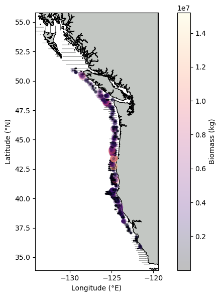
We can pass a few keyword arguments to modify the behavior of the scatterplot points, such as the color and transparency:

egra.plot_transect_map(
    data=df_nasc_all_ages,
    variable="biomass",
    axis_kwargs={"xlabel": "Longitude (\u00b0E)", "ylabel": "Latitude (\u00b0N)"},
    colorbar_kwargs={"label": "Biomass (kg)", "cmap": "magma"},
    scatter_kwargs={"alpha": 0.25, "cmap": "magma"},
    plot_kwargs={"figsize": (8, 6)},
)

C:\Users\Brandyn Lucca\Documents\GitHub\echopop\echopop\nwfsc_feat\graphics\utils.py:118: UserWarning: The following keys were not accepted by 'NaturalEarthFeature' and were pruned: ['edgecolor', 'facecolor']
  coast_feature = call_with_pruned(
C:\Users\Brandyn Lucca\Documents\GitHub\echopop\echopop\nwfsc_feat\graphics\transect_map.py:226: UserWarning: The following keys were not accepted by 'axes' and were pruned: ['extent']
  ax = gutils.call_with_pruned(plt.axes, {"extent": [x0, x1, y0, y1], **axis_kwargs})

Modifying the coast and transect lines

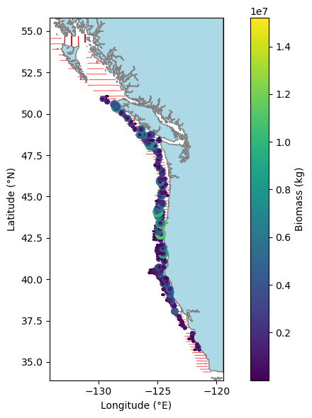
We can also modify the behavior of the coastline and transect lines:

egra.plot_transect_map(
    data=df_nasc_all_ages,
    variable="biomass",
    axis_kwargs={"xlabel": "Longitude (\u00b0E)", "ylabel": "Latitude (\u00b0N)"},
    colorbar_kwargs={"label": "Biomass (kg)"},
    coast_kwargs={"edgecolor": "gray", "facecolor": "lightblue"},
    transect_kwargs={"color": "red"},
    plot_kwargs={"figsize": (8, 6)},
)

C:\Users\Brandyn Lucca\Documents\GitHub\echopop\echopop\nwfsc_feat\graphics\utils.py:118: UserWarning: The following keys were not accepted by 'NaturalEarthFeature' and were pruned: ['edgecolor', 'facecolor']
  coast_feature = call_with_pruned(
C:\Users\Brandyn Lucca\Documents\GitHub\echopop\echopop\nwfsc_feat\graphics\transect_map.py:226: UserWarning: The following keys were not accepted by 'axes' and were pruned: ['extent']
  ax = gutils.call_with_pruned(plt.axes, {"extent": [x0, x1, y0, y1], **axis_kwargs})

Kriged mesh results

Spatial distributions of kriged variables can be visualized via plot_kriged_mesh. This expects a pandas.DataFrame or geopandas.GeoDataFrame comprising appropriate coordinates (e.g. longitude, latitude). The plot_kriged_mesh function has many arguments that can configure the table to one’s preferences.

• data: The input pandas.DataFrame or geopandas.GeoDataFrame with coordinates and desired variable for plotting.

• variable: The name of the column within the DataFrame/GeoDataFrame to plot.

• projection: The CRS (e.g. "epsg:4326") that should either be a projected or geodetic coordinate system copmatible with the geopandas.GeoDataFrame-class.

• coordinate_names: This is a tuple comprising the coordinate names (i.e. columns within the DataFrame/GeoDataFrame) with an expected order of ‘horizontal’ followed by ‘vertical’. For instance, this may look like ("longitude", "latitude") or ("x", "y").

• plot_type: Type of plot to produce. Options are:

  • "hexbin": Creates a hexagonal binned plot using matplotlib.pyplot.hexbin, which visualizes a summary statistic defined by the user (via the reduce_C_function argument, which defaults to numpy.mean) over a two-dimensional grid of hexagons. The plotted hexagonal bins can be configured using keyword arguments supplied to the hexbin_kwargs argument.

  • "pcolormesh": Interpolates the variable onto a regular grid using interpolation_mesh, which internally leverages the verde library for spatial ineroplation that returns an xarray.DataArray object. The resulting grid is then displayed as a pseudcolor mesh using xarray.DataArray.plot.pcolormesh. The plotted pseudocolor mesh can be configured using keyword arguments supplied to the pseudocolormesh_kwargs argument.

  • "scatter": Plots each data point individually using matplotlib.axes.Axes.scatter color poitns based on the variabel value. The plotted points can be configured using keyword arguments supplied to the scatter_kwargs argument.

• scatter_kwargs: Keyword arguments for matplotlib.axes.Axes.scatter.

• hexbin_kwargs: Keyword arguments for matplotlib.pyplot.hexbin.

• pseudocolormesh_kwargs: Keyword arguments for xarray.DataArray.plot.pcolormesh.

• coast_kwargs: Keyword arguments for cartopy.feature.NaturalEarthFeature used for coastline plotting.

• axis_kwargs: Keyword arguments for axis formatting (e.g. labels) used by matplotlib.pyplot.

• plot_kwargs: Keyword arguments used by matplotliib.pyplot.subplots.

• colorbar_kwargs: Keyword arguments for matplotlib.pyplot.colorbar.

• save_path: A pathlib.Path object defining the filepath for where the figure should be saved.

• savefig_kwargs: Keyword arguments for matplotlib.pyplot.savefig.

Basic plotting

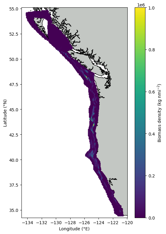
The most basic version of this plot can be generated via:

egra.plot_kriged_mesh(
    data=unextrapolated_results,
    variable="biomass_density",
    axis_kwargs={"xlabel": "Longitude (\u00b0E)", "ylabel": "Latitude (\u00b0N)"},
    colorbar_kwargs={"label": r"Biomass density (kg $\mathregular{nmi^{-2}}$)"},
    savepath=SAVE_DIRECTORY / "kriged_mesh_hexbin_base.png"
)

C:\Users\Brandyn\GitHub\echopop\echopop\graphics\utils.py:118: UserWarning: The following keys were not accepted by 'NaturalEarthFeature' and were pruned: ['edgecolor', 'facecolor']
  coast_feature = call_with_pruned(

Like earlier, we can adjust the vmin and vmax scaling, along with other colorbar-specific arguments, to help visualize the variability in our interpolated field:

# Define scale 
norm = SymLogNorm(linthresh=1., vmin=0., vmax=unextrapolated_results.biomass_density.max())

# Create colormap
scaled_colormap = plt.cm.ScalarMappable(norm=norm, cmap="cividis")

# Plot
egra.plot_kriged_mesh(
    data=unextrapolated_results,
    variable="biomass_density",
    axis_kwargs={"xlabel": "Longitude (\u00b0E)", "ylabel": "Latitude (\u00b0N)"},
    colorbar_kwargs={"label": r"Biomass density (kg $\mathregular{nmi^{-2}}$)",
                     "mappable": scaled_colormap},
    hexbin_kwargs={"norm": norm, "cmap": "cividis"},
    savepath=SAVE_DIRECTORY / "kriged_mesh_hexbin_base.png"
)


    

C:\Users\Brandyn\GitHub\echopop\echopop\graphics\utils.py:118: UserWarning: The following keys were not accepted by 'NaturalEarthFeature' and were pruned: ['edgecolor', 'facecolor']
  coast_feature = call_with_pruned(

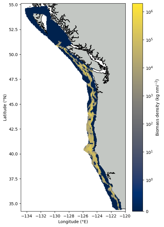
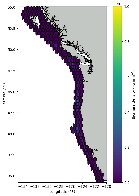
The default plot_type is hexbin, which here shows the mean biomass density for each hexagonal bin.

Adjusting the hexagonal binning

The hexagonal bins can be adjusted in several ways. For instance, one can select a new grid size for the hexagons to be computed over:

egra.plot_kriged_mesh(
    data=unextrapolated_results,
    variable="biomass_density",
    hexbin_kwargs={"gridsize": 50, "edgecolors": "black"},
    axis_kwargs={"xlabel": "Longitude (\u00b0E)", "ylabel": "Latitude (\u00b0N)"},
    colorbar_kwargs={"label": r"Biomass density (kg $\mathregular{nmi^{-2}}$)"},
)

C:\Users\Brandyn\GitHub\echopop\echopop\graphics\utils.py:118: UserWarning: The following keys were not accepted by 'NaturalEarthFeature' and were pruned: ['edgecolor', 'facecolor']
  coast_feature = call_with_pruned(

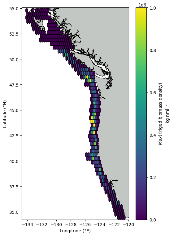
Alternatively, the metrics other than the mean can be supplied, such as the maximum value in each hexagon:

import numpy as np

egra.plot_kriged_mesh(
    data=unextrapolated_results,
    variable="biomass_density",
    hexbin_kwargs={"gridsize": 50, "edgecolors": "black", "reduce_C_function": np.max},
    axis_kwargs={"xlabel": "Longitude (\u00b0E)", "ylabel": "Latitude (\u00b0N)"},
    colorbar_kwargs={"label": "$Max$(Kriged biomass density)\nkg nmi$^{-2}$"},
)

C:\Users\Brandyn Lucca\Documents\GitHub\echopop\echopop\nwfsc_feat\graphics\utils.py:118: UserWarning: The following keys were not accepted by 'NaturalEarthFeature' and were pruned: ['edgecolor', 'facecolor']
  coast_feature = call_with_pruned(

Scatter plot.

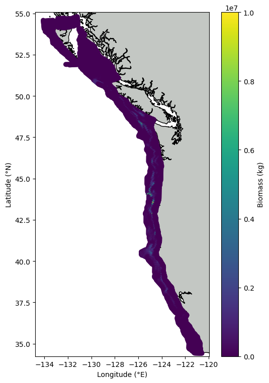
Using plot_type = "scatter" produces “simplest” plot that will likely render quicker than the other two types for smaller datasets:

egra.plot_kriged_mesh(
    data=unextrapolated_results,
    variable="biomass",
    plot_type="scatter",
    axis_kwargs={"xlabel": "Longitude (\u00b0E)", "ylabel": "Latitude (\u00b0N)"},
    colorbar_kwargs={"label": "Biomass (kg)"},
)

C:\Users\Brandyn Lucca\Documents\GitHub\echopop\echopop\nwfsc_feat\graphics\utils.py:118: UserWarning: The following keys were not accepted by 'NaturalEarthFeature' and were pruned: ['edgecolor', 'facecolor']
  coast_feature = call_with_pruned(

This will accept similar keyword arguments as those described for the plot_age_length_heatmap function above.

Adjusting the pseudocolor mesh

Alternatively, these data can be interpolated to generate a pseudocolor plot via a nearest-neighbors algorithm. This can be helpful for visualizing broader spatial trends where data may be sparse or otherwise noisy:

egra.plot_kriged_mesh(
    data=unextrapolated_results,
    variable="biomass",
    plot_type="pcolormesh",
    axis_kwargs={"xlabel": "Longitude (\u00b0E)", "ylabel": "Latitude (\u00b0N)"},
    colorbar_kwargs={"label": "Biomass (kg)"},
)

C:\Users\Brandyn Lucca\Documents\GitHub\echopop\echopop\nwfsc_feat\graphics\utils.py:118: UserWarning: The following keys were not accepted by 'NaturalEarthFeature' and were pruned: ['edgecolor', 'facecolor']
  coast_feature = call_with_pruned(

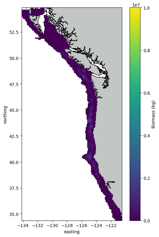
The spatial extent of the interpolation can be adjusted via pseudocolormesh_kwargs where the keyword argument "spacing" is in degrees. So for instance, "spacing": 0.01 means that the interpolator smooths values over a 0.01 degree increment in all directions around each point:

egra.plot_kriged_mesh(
    data=unextrapolated_results,
    variable="biomass",
    plot_type="pcolormesh",
    axis_kwargs={"xlabel": "Longitude (\u00b0E)", "ylabel": "Latitude (\u00b0N)"},
    colorbar_kwargs={"label": "Biomass (kg)"},
    pseudocolormesh_kwargs={"spacing": 0.01}
)

C:\Users\Brandyn Lucca\Documents\GitHub\echopop\echopop\nwfsc_feat\graphics\utils.py:118: UserWarning: The following keys were not accepted by 'NaturalEarthFeature' and were pruned: ['edgecolor', 'facecolor']
  coast_feature = call_with_pruned(

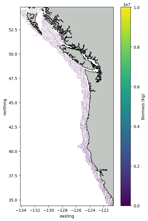
egra.plot_kriged_mesh(
    data=unextrapolated_results,
    variable="biomass",
    plot_type="pcolormesh",
    axis_kwargs={"xlabel": "Longitude (\u00b0E)", "ylabel": "Latitude (\u00b0N)"},
    colorbar_kwargs={"label": "Biomass (kg)"},
    pseudocolormesh_kwargs={"spacing": 0.05}
)

C:\Users\Brandyn Lucca\Documents\GitHub\echopop\echopop\nwfsc_feat\graphics\utils.py:118: UserWarning: The following keys were not accepted by 'NaturalEarthFeature' and were pruned: ['edgecolor', 'facecolor']
  coast_feature = call_with_pruned(

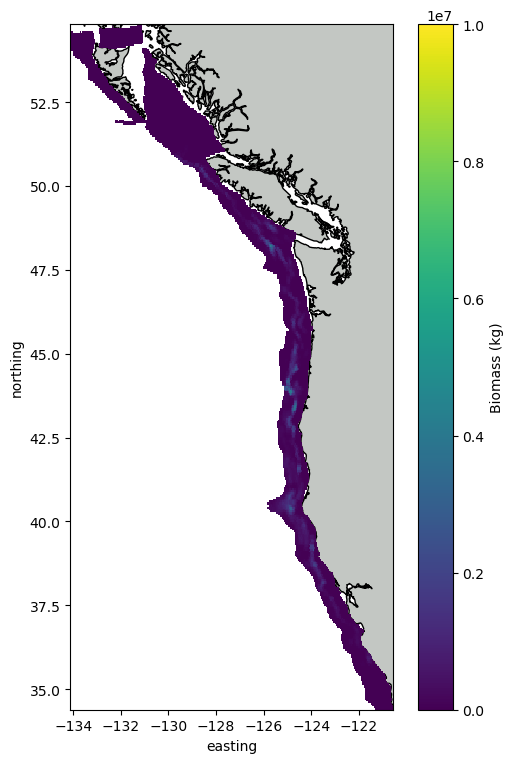
egra.plot_kriged_mesh(
    data=unextrapolated_results,
    variable="biomass",
    plot_type="pcolormesh",
    axis_kwargs={"xlabel": "Longitude (\u00b0E)", "ylabel": "Latitude (\u00b0N)"},
    colorbar_kwargs={"label": "Biomass (kg)"},
    pseudocolormesh_kwargs={"spacing": 0.1}
)

C:\Users\Brandyn Lucca\Documents\GitHub\echopop\echopop\nwfsc_feat\graphics\utils.py:118: UserWarning: The following keys were not accepted by 'NaturalEarthFeature' and were pruned: ['edgecolor', 'facecolor']
  coast_feature = call_with_pruned(

egra.plot_kriged_mesh(
    data=unextrapolated_results,
    variable="biomass",
    plot_type="pcolormesh",
    axis_kwargs={"xlabel": "Longitude (\u00b0E)", "ylabel": "Latitude (\u00b0N)"},
    colorbar_kwargs={"label": "Biomass (kg)"},
    pseudocolormesh_kwargs={"spacing": 0.5}
)

C:\Users\Brandyn Lucca\Documents\GitHub\echopop\echopop\nwfsc_feat\graphics\utils.py:118: UserWarning: The following keys were not accepted by 'NaturalEarthFeature' and were pruned: ['edgecolor', 'facecolor']
  coast_feature = call_with_pruned(