
Correct proportions for net selectivity#
Import necessary modules#
With the number proportions calculated, we can optionally correct them for length-based net selectivity. This is done via the selectivity module of the survey sub-package.
from echopop.survey import selectivity, proportions
Net selectivity diverges from the standard workflow at the count-binning stage. Selectivity expansion is applied before tabulating counts and number proportions, and weight proportions are then derived from those corrected number proportions using fitted length-binned weights.
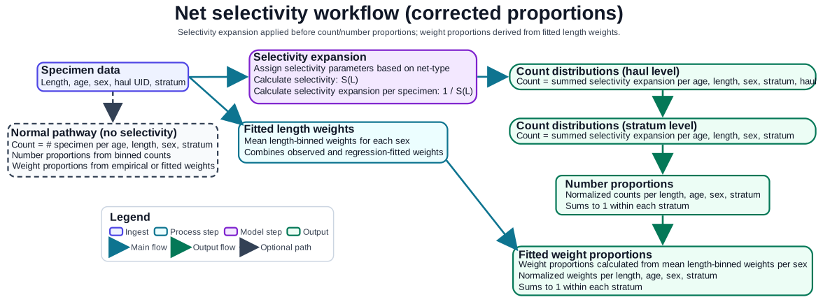
Assigning selectivity expansion factors#
In the selectivity pathway, corrections are applied at the specimen level before any stratum-level normalization. If \(S(L_i)\) is the retention probability for specimen \(i\) at length \(L_i\), then the effective selectivity expansion factor can be assigned to each animal. The key function in this step is assign_selectivity_expansion.
Core arguments are:
biodata: Specimen-levelpandas.DataFramecontaining at least length and net-type columns.net_selectivity_params: Selectivity parameters in one of two accepted formats.net_column: Name of the net-type column used to map parameters (for example,"gear").minimum_selectivity: Numerical floor \(S_{\min}\) used to stabilize inverse weighting.
net_selectivity_params supports both of the following structures:
Single global parameter set (applies the same ogive to all nets):
{"l50": 10.9, "sr": 14.0}
Net-specific parameter dictionary (different parameters by net/gear type):
{
    "AWT": {"l50": 10.9, "sr": 14.0},
    "IKMT": {"intercept": -8.2, "slope": 0.58},
}
Each parameter block must be either (l50, sr) or (intercept, slope). This allows mixed parameterization across net types while still mapping to the same logistic selectivity formulation.
Preparing the data#
For this example, we will only consider the specimen-specific data since that is the intended data format.
specimen_data = dict_df_bio["specimen"]
We can inspect the catch data to see the various (or singular) net-types used during the survey.
dict_df_bio["catch"].gear.unique()
array(['AWT'], dtype=object)
However, specimen_data does not contain this column:
"gear" in specimen_data
False
Since the "gear" column does not exist in specimen_data, we have to merge that information from dict_df_bio["catch"]:
specimen_data = dict_df_bio["specimen"].merge(
    dict_df_bio["catch"][["uid", "gear"]].drop_duplicates("uid"),
    on="uid",
    how="left",
)
We can now see that specimen_data contains this column:
"gear" in specimen_data
True
specimen_data["gear"].unique()
array(['AWT'], dtype=object)
Assigning expansion factors to each row#
Since only one net-type is present in specimen_data, the NET_SELECTIVITY_GLOBAL dictionary can be used since it will uniformly apply those parameters across all rows:
# Apply selectivity expansion at the specimen level using the selected NET_SELECTIVITY definition
specimen_data_selectivity = selectivity.assign_selectivity_expansion(
    specimen_data,
    NET_SELECTIVITY_GLOBAL,
    net_column="gear",
    minimum_selectivity=1e-12,
)
The output pandas.DataFrame now has three additional columns: l50, sr, and selectivity_expansion
specimen_data_selectivity.filter(["sex", "length", "uid", "gear", "l50", "sr", "selectivity_expansion"])
| sex | length | uid | gear | l50 | sr | selectivity_expansion | |
|---|---|---|---|---|---|---|---|
| 0 | male | 24.0 | 2-2-99999-1.0 | AWT | 10.9 | 14.0 | 1.067928 |
| 1 | female | 23.0 | 2-2-99999-1.0 | AWT | 10.9 | 14.0 | 1.184647 |
| 2 | female | 22.0 | 2-2-99999-1.0 | AWT | 10.9 | 14.0 | 1.501923 |
| 3 | male | 22.0 | 2-2-99999-1.0 | AWT | 10.9 | 14.0 | 1.501923 |
| 4 | female | 23.0 | 2-2-99999-1.0 | AWT | 10.9 | 14.0 | 1.184647 |
| ... | ... | ... | ... | ... | ... | ... | ... |
| 3260 | female | 46.0 | 2-2-99999-222.0 | AWT | 10.9 | 14.0 | 1.000000 |
| 3261 | female | 46.0 | 2-2-99999-222.0 | AWT | 10.9 | 14.0 | 1.000000 |
| 3262 | female | 52.0 | 2-2-99999-222.0 | AWT | 10.9 | 14.0 | 1.000000 |
| 3263 | female | 48.0 | 2-2-99999-222.0 | AWT | 10.9 | 14.0 | 1.000000 |
| 3264 | male | 49.0 | 2-2-99999-222.0 | AWT | 10.9 | 14.0 | 1.000000 |
3265 rows × 7 columns
Converting to corrected number proportions#
These selectivity expansion factors are first summed across all indices including the haul-level identifier uid. This is to maintain good habits since there may be cases where a dataset has multiple net-types that will map different selectivity parameters to specific haul numbers.
# Effective counts per haul (length × age × sex × stratum × uid)
da_count_distribution_hauls = proportions.compute_binned_counts(
    data=specimen_data_selectivity.dropna(subset=["length"]),
    groupby_cols=["stratum_ks", "length_bin", "age_bin", "sex", "uid"],
    count_col="selectivity_expansion",
    agg_func="sum",
)
These can then be summed over each stratum:
# Collapse to stratum level
da_count_distribution_strata = da_count_distribution_hauls.sum(dim=["uid"])
The last step is then to normalize these effective counts by converting them into proportions:
ds_number_proportions_corrected = proportions.number_proportions(
    data=da_count_distribution_strata,
    stratum_dim="stratum_ks",
    exclude_filters={"sex": "unsexed"},
)
<xarray.Dataset> Size: 255kB
Dimensions:     (stratum_ks: 9, length_bin: 40, age_bin: 22, sex: 2)
Coordinates:
  * stratum_ks  (stratum_ks) int64 72B 0 1 2 3 4 5 6 7 8
  * length_bin  (length_bin) category 680B (1.0, 3.0] ... (79.0, 81.0]
  * age_bin     (age_bin) category 374B (0.5, 1.5] (1.5, 2.5] ... (21.5, 22.5]
  * sex         (sex) object 16B 'female' 'male'
Data variables:
    count       (stratum_ks, length_bin, age_bin, sex) float64 127kB 0.0 ... 0.0
proportion (stratum_ks, length_bin, age_bin, sex) float64 127kB 0.0 ... 0.0The corrected output is an xarray.Dataset returned by proportions.number_proportions. It retains the original dimensional structure (typically stratum × length_bin × age_bin × sex), but with selectivity-adjusted effective counts embedded in the normalization. In practice, one variable is central: proportion (overall normalized proportions for downstream weighting and slicing operations). When within-group proportions are needed, they can be derived by re-normalizing proportion within the target group context. If age is absent in the source specimen records, the output naturally reduces to a length-based structure. The differences in the selectivity-corrected and uncorrected number proportions for a few example strata show how the adjustment varies depending on the length range a stratum comprises.
Converting to corrected weight proportions#
After corrected number proportions are obtained, weight proportions are computed by combining those corrected distributions with fitted mean length-binned weights. In this workflow (combined aged/unaged pathway), Echopop uses fitted_weight_proportions_combined.
Conceptually, corrected number proportions define the conditional composition across age/sex within each length bin, while fitted length weights provide the length-marginal mass scaling. The resulting dataset is re-normalized within each stratum and remains dimensionally compatible with downstream abundance and biomass apportionment.
The key function in this step is fitted_weight_proportions_combined, with core arguments:
number_proportions: Corrected number-proportionxarray.Datasetcontainingproportion.binned_weights: Fitted length-binned weights aligned onlength_bin(typicallysex="all"weights).stratum_dim: Stratum dimensions that define normalization groups (e.g.,["stratum_ks"]).
# Derive weight proportions from selectivity-corrected number proportions using fitted length-binned weights
ds_weight_proportions_corrected = proportions.fitted_weight_proportions_combined(
    number_proportions=ds_number_proportions_corrected,
    binned_weights=da_binned_weights_all,
    stratum_dim="stratum_ks",
)
<xarray.Dataset> Size: 1kB
Dimensions:     (stratum_ks: 9, length_bin: 40, age_bin: 22, sex: 0)
Coordinates:
  * stratum_ks  (stratum_ks) int64 72B 0 1 2 3 4 5 6 7 8
  * length_bin  (length_bin) category 680B (1.0, 3.0] ... (79.0, 81.0]
  * age_bin     (age_bin) category 374B (0.5, 1.5] (1.5, 2.5] ... (21.5, 22.5]
  * sex         (sex) object 0B
Data variables:
proportion (stratum_ks, length_bin, age_bin, sex) float64 0B The output is an xarray.Dataset with the data variable proportion, representing weight-scaled proportions that sum to 1 within each stratum under the provided stratum_dim definition. Because the calculation is driven by corrected number proportions, the age/sex/length structure remains coherent with the corrected count pathway.
Integrating into the general workflow#
With ds_number_proportions_corrected and ds_weight_proportions_corrected computed, the net-selectivity pathway can be dropped into the same downstream steps used by the standard FEAT workflow: abundance apportionment, biomass apportionment, age filters, and geostatistical projection. The only structural difference is where correction enters the pipeline (specimen-level expansion before count tabulation).